4376

Flow Quantification for Cerebrospinal Fluid by Spatial-temporal Perturbation Patterns in SSFP

Yicun Wang¹, Peter van Gelderen¹, Jacco A. de Zwart¹, Pinar S. Özbay¹, Hendrik Mandelkow¹, Dante Picchioni¹, and Jeff H. Duyn¹
¹AMRI, LFMI, NINDS, National Institutes of Health, Bethesda, MD, United States

Synopsis

We report a fast quantitative CSF flow imaging method based on the spatial-temporal perturbation patterns formed at the transition bands in balanced steady-state-free-precession (SSFP) images when combined with a background magnetic field gradient. By modeling CSF flow as a combination of a pulsatile (AC) and a constant (DC) flow component across the cardiac cycle, a dictionary was generated based on Bloch simulations and used to translate the observed patterns to flow velocities. Monte-Carlo simulations were performed to evaluate the accuracy of the approach. CSF flow resulting from different physiological mechanisms was quantified in selected regions in 12 healthy subjects.

Introduction

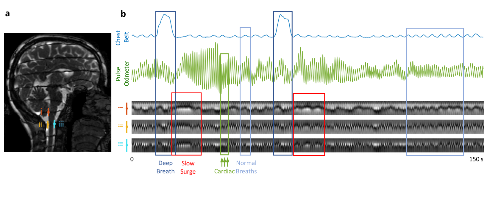
CSF pulsations may facilitate glymphatic clearance of metabolic waste products from the brain, and thus may play a role in alleviation of neurodegeneration that leads to Alzheimer’s Disease (1,2). Quantification of CSF flow has been performed by phase-contrast MRI (3–6), and also by inversion labelling methods (7), from which it is understood that CSF pulsations are primarily driven by passive vascular response to blood pressure variations associated with cardiac and respiratory cycles. Nevertheless, existing methods provide rather limited precision because of the low CSF flow velocities (1-20 mm/s). Additionally, other flow types may exist that evade detection by the event-locked imaging or analysis approaches, especially those not synchronized with cardiac and respiratory cycles.
Recently, Oshio et al. proposed that CSF flow could be qualitatively visualized using continuously acquired balanced steady state free precession (SSFP) images when combined with a background magnetic field gradient that creates dark bands across the image (8). Using this approach, we observed not only band movement associated with cardiorespiratory effects, but also slow movement following intermittent deep inspirations (Figure 1). Their timing was consistent with a cerebral autoregulation mechanism (9,10). We sought to translate the observed CSF “perturbation patterns” to velocity values by means of dictionary searching, and to estimate the relative strength of the previously undetected slow component compared to the cardiorespiratory effects.

Methods

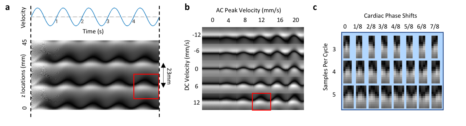
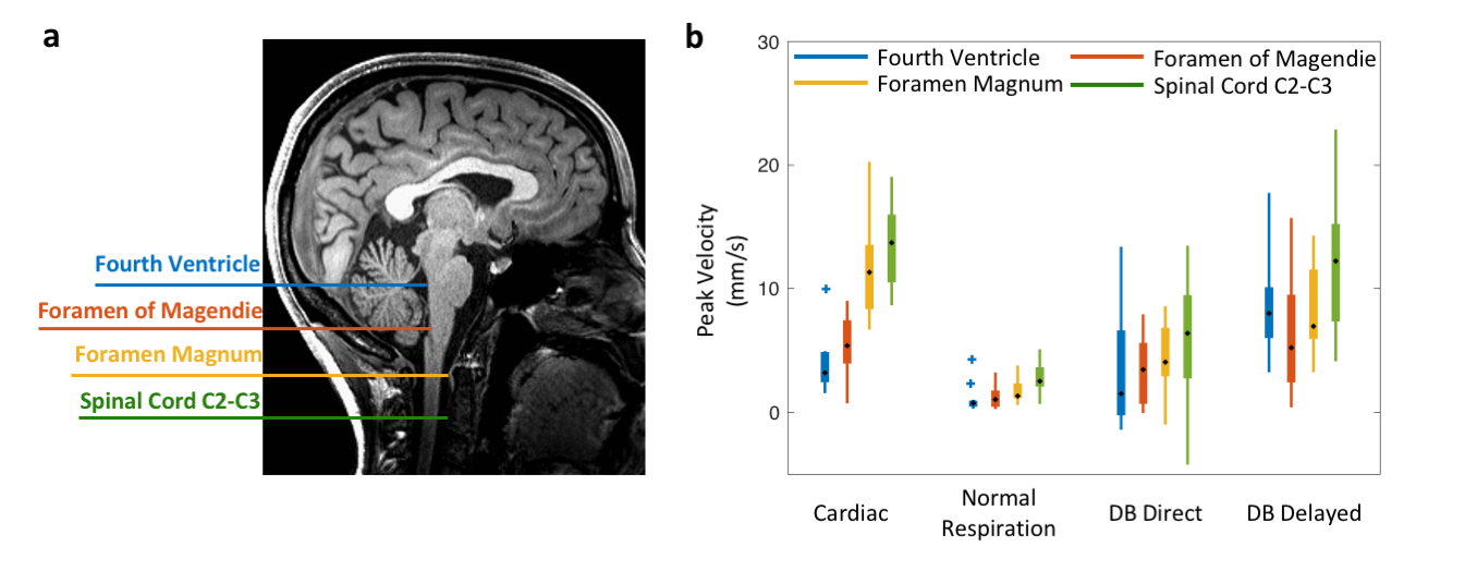
MRI experiments 12 healthy volunteers were scanned in a 3 T Prisma using a 64-channel receive array (Siemens Healthineers, Erlangen, Germany). Parameters: single sagittal slice of 3 mm thickness, TR 6 ms, TE 3 ms, FA 45°, SENSE 3, FOV 240×204 mm², resolution 1.3×1.7 mm², bandwidth 250 kHz, slice TR 246 ms. A background z gradient of ~0.17 mT/m was added by manually adjusting the shim current, creating bands that were ~23 mm apart. Subjects were visually instructed to take a deep breath every 50 s, skipping every 3rd one. The entire run was 7.5 min containing 6 deep breaths. Respiration and cardiac rhythms were recorded using a chest belt and a finger pulse oximeter respectively, sampled at 2 kHz (Biopac, Goleta, CA, USA).
Dictionary CSF flow within each cardiac cycle may be modelled as a combination of a sinusoid (cardiac) and constant (slower than cardiac, e.g. respiratory) flow component. We refer to these as AC and DC components in analogy to electrical circuits. Bloch simulations were performed to obtain spatial-temporal (i.e. band profile-time) perturbation patterns corresponding to stepped AC peak velocities (0 – 60 mm/s with 1 mm/s steps) and DC velocities (-40 – 40 mm/s with 1 mm/s steps) (Figure. 2). T₁ and T₂ of CSF were assumed to be 4 and 2 s. To account for phase differences between the simulation and in-vivo data, the simulated perturbation patterns were phase cycled by 8 steps. The patterns were then downsampled to either 3, 4, or 5 time points to match cardiac periods of around 0.75, 1.00 and 1.25 s. The total number of dictionary entries was thus 61×81×8×3=118,584.
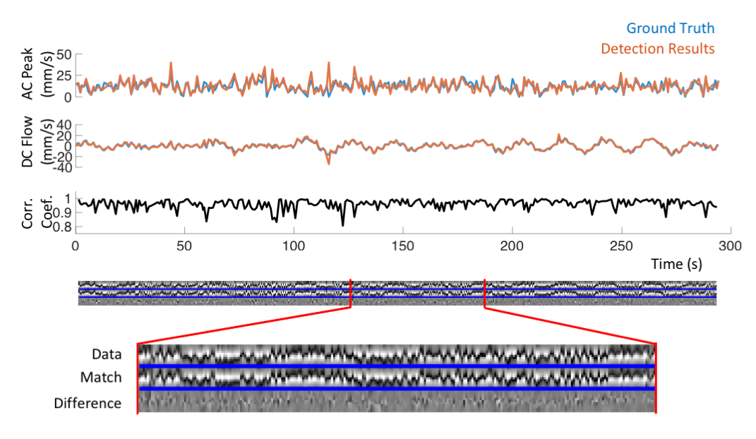
Monte-Carlo simulations We numerically generated data from 500 runs of about 300 s each, comprising 3 physiologically relevant frequency components with randomized periods and amplitudes (periods 1.0±0.2, 3.5±0.5, 20±1 s, peak velocities 12±6, 4±2, 8±5 mm/s). The detection method used for the in vivo data was applied as described below.
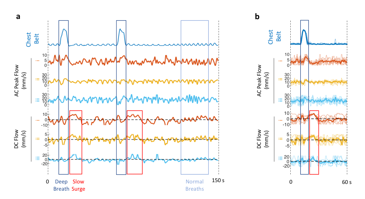
In-vivo data analysis The temporal changes of manually selected band profiles (11 voxels long) along the CSF canal (e.g. those in Figure 1b) were segmented into perturbation patterns corresponding to each cardiac cycle based on the finger pulse oximeter signal. The perturbation patterns were then matched to the dictionary using correlation coefficient as the metric, similar to MR Fingerprinting (11). Velocity estimation for the flow associated with the cardiac cycle was performed by averaging AC results, while those with respiratory and slow surges were based on peak detection of DC results.

Results

Detection results closely followed the ground truth in Monte-Carlo simulations (Figure 3). Over 147,482 simulated cardiac cycles, the estimation error in AC was 0.66±5.26 mm/s and that in DC was 0.32±3.35 mm/s (mean±std). For in-vivo detection, results from different CSF locations showed similar temporal features associated with respiration (Figure 4a). The slow surge after a deep breath observed on the perturbation patterns was also clear on the quantitative results (Figure 4b). In the group analysis results (Figure 5), cardiac and respiratory effects were similar to previous findings (5,6). In addition, the novel low-frequency flow has comparable peak velocities to the cardiac effect, with less location dependency.

Conclusion

We developed a CSF flow quantification method using a dictionary approach for the spatial-temporal changes of the transition bands on SSFP images. Monte-Carlo simulations demonstrated reasonable accuracy (standard deviation of 3 – 5 mm/s) of the approach for physiologically relevant CSF flow velocities. In a group of 12 control subjects, velocities associated with cardiorespiratory effects were similar to previous studies. Additionally, we quantified a novel low-frequency flow after a deep breath. The relative importance of this novel component to CSF mixing, and eventually brain waste clearance remains to be investigated. The proposed approach may be helpful in characterization of the CSF flow dynamics associated with the various mechanisms.

Acknowledgements

This study was supported by the intramural program of NINDS, NIH.

References

1. Iliff JJ, Wang M, Liao Y, et al. A Paravascular Pathway Facilitates CSF Flow Through the Brain Parenchyma and the Clearance of Interstitial Solutes, Including Amyloid β. Sci. Transl. Med. 2012;4:147ra111-147ra111.

2. Plog BA, Nedergaard M. The Glymphatic System in Central Nervous System Health and Disease: Past, Present, and Future. Annu. Rev. Pathol. Mech. Dis. 2018;13:379–394.

3. Feinberg DA, Mark AS. Human brain motion and cerebrospinal fluid circulation demonstrated with MR velocity imaging. Radiology 1987;163:793–799.

4. Alperin N, Vikingstad EM, Gomez‐Anson B, Levin DN. Hemodynamically independent analysis of cerebrospinal fluid and brain motion observed with dynamic phase contrast MRI. Magn. Reson. Med. 1996;35:741–754.

5. Chen L, Beckett A, Verma A, Feinberg DA. Dynamics of respiratory and cardiac CSF motion revealed with real-time simultaneous multi-slice EPI velocity phase contrast imaging. NeuroImage 2015;122:281–287.

6. Yildiz S, Thyagaraj S, Jin N, et al. Quantifying the influence of respiration and cardiac pulsations on cerebrospinal fluid dynamics using real-time phase-contrast MRI. J. Magn. Reson. Imaging 2017;46:431–439.

7. Yamada S, Miyazaki M, Kanazawa H, et al. Visualization of Cerebrospinal Fluid Movement with Spin Labeling at MR Imaging: Preliminary Results in Normal and Pathophysiologic Conditions. Radiology 2008;249:644–652.

8. Oshio K, Yui M, Shimizu S, Yamada S. Continuously visualizing slow flow using SSFP. In: Proc. Intl. Soc. Mag. Reson. Med. 27, Montréal, 2019, p. 2974. ; 2019.

9. Özbay PS, Chang C, Picchioni D, et al. Sympathetic activity contributes to the fMRI signal. Commun. Biol. 2019;2:1–9.

10. Picchioni D, Özbay PS, Mandelkow H, et al. Autonomic arousals contribute to brain fluid pulsations during sleep. bioRxiv 2021:2021.05.04.442672.

11. Ma D, Gulani V, Seiberlich N, et al. Magnetic resonance fingerprinting. Nature 2013;495:187–192.

Figures

Figure 1. Band movement along the CSF canal in SSFP images correpsonds to multiple physiological mechanisms. (a) An example SSFP image acquired with a background z gradient showing equidistant dark bands in the head and neck. (b) Plots of band profiles across time at the 3 locations labeled in (a), and the corresponding peripheral physiological signals. In addition to the known cardiac and respiratory effects on CSF flow that create pulsatile band movement, slow surges of CSF can also be observed especially after a deep breath.

Figure 2. Dictionary generation by Bloch simulations of flowing spins. (a) Simulated spatial-temporal signal changes using a constant flow (DC) of 12 mm/s and a pulsatile flow (AC) of 1 s period and 12 mm/s peak velocity. The red box outlines a converged pattern for further processing. (b) A subset of converged patterns that are characteristic for different AC and DC settings. (c) Each pattern was phase-cycled to accommodate phase differences between simulated and exprimental data, and subsampled in time and space to match imaging resolutions.

Figure 3. An example Monte-Carlo simulation result. Blue is the ground truth, i.e. AC and DC values used to simulate flow patterns, and orange is detection results. Corr. Coef.: correlation coefficient. The data of the entire run is shown, together with the best match concatenating those for all cardiac cycles, and their difference. A section is zoomed in for visualization.

Figure 4. In-vivo detection results. (a) AC and DC results for the perturbation patterns shown in Figure 1b. (b) Superposition of 6 data segments (thin lines) in one run (time locked at the end of deep inspiration), as well as their avearge (thick lines).

Figure 5. CSF peak velocities by different mechanisms at four different locations along the CSF canal. Data from 12 control subjects are shown. The central dot represents median; the upper (lower) edge of box represents the 1st (3rd) quartile; whiskers extend to extremes within twice the inter-quartile interval; “+” represents outliers. DB: deep breaths.

Proc. Intl. Soc. Mag. Reson. Med. 30 (2022)

4376

DOI: https://doi.org/10.58530/2022/4376