Introduction

The calculation and analysis of magnetic field and magnetic force among permanent magnets are critical to magnet array designs for different purposes, e.g., for portable dedicated magnetic resonance imaging(MRI) system where arrays consist of cuboid magnets[1-3], motor designs[4-5], etc. Most studies use numerical simulation software to compute the magnetic field for designs[1-3]. However, it has the following problems. First, the accuracy of numerical simulations highly depends on the simulation settings, such as the boundary setup. Second, a high simulation accuracy is usually obtained at a price of high time and memory consumption[6]. This can make a magnet array optimization with a high design flexibility impractical , which usually involves many magnets and where one simulation can take several hours, and hundreds of simulations are required before reaching the optimum. To address these problems and to accelerate magnet array optimizations, we propose a magnet simulator that performs fast calculation for both magnetic field and magnetic force in permanent magnet arrays, focusing on those that consists of cuboid magnets that are available off-the-shelf, targeting on magnet array optimizations for portable MRI.

Method

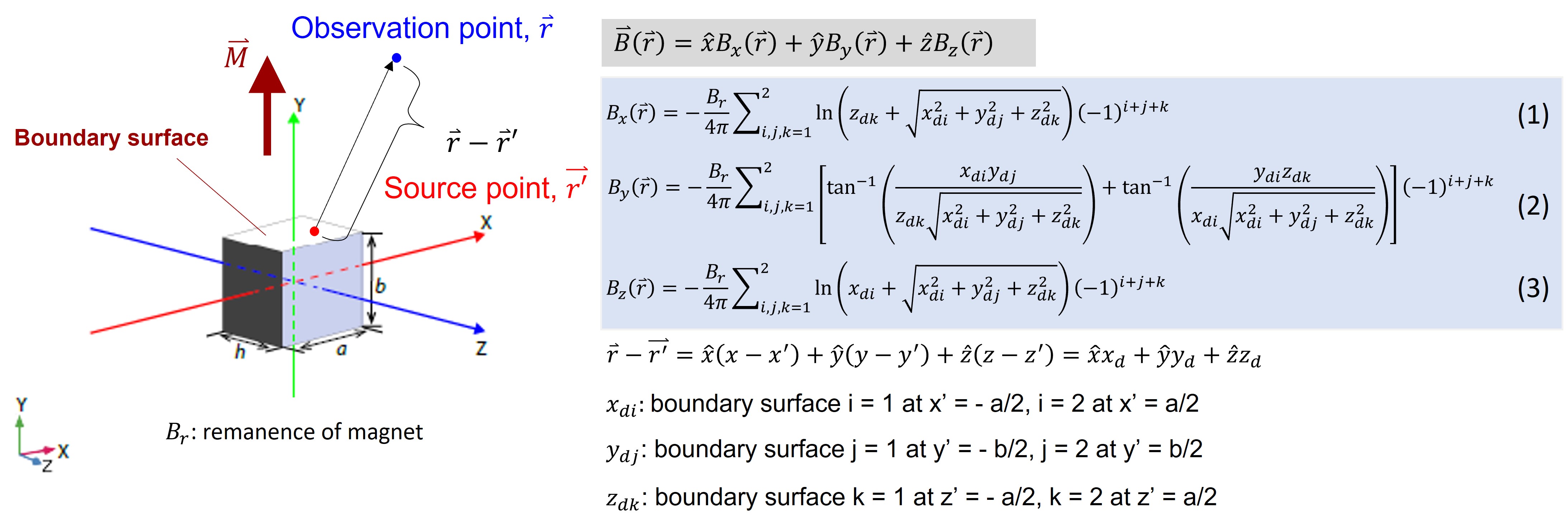
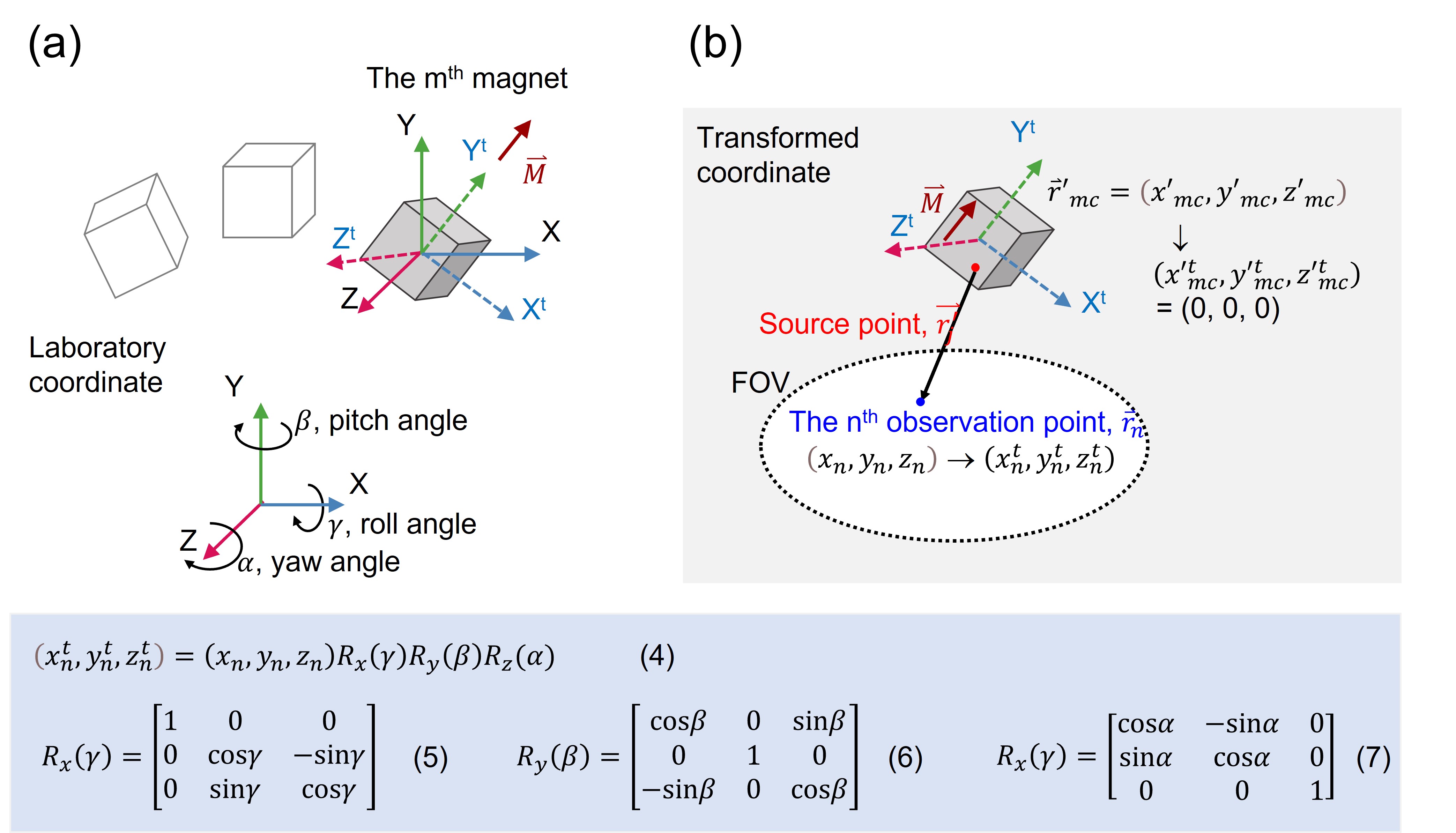
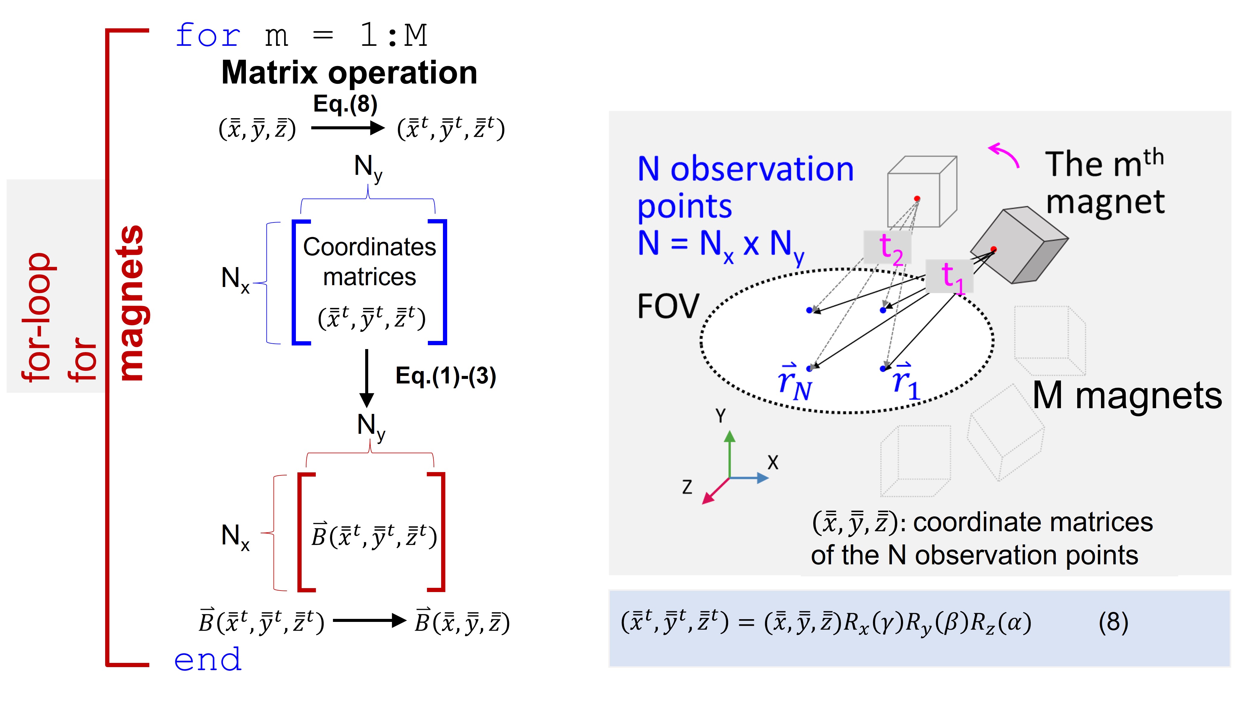
The calculation of magnetic field produced by magnets is based on the current-based model[7]. Fig.1 shows the formulation (Eq.(1)-(3)) for a y-polarized magnet centered at the origin. This formulation can still be used to calculate the magnetic field (the n^th observation point in the field-of-view (FoV) denoted as $$$\vec{r}_n(x_n,y_n,z_n)$$$) of a magnet arbitrarily off the origin at $$$(x'_{mc},y'_{mc},z'_{mc})$$$ when transformation of coordinates shown in Fig.2(a) is applied. It is defined by transforming the y-polarized magnet at the laboratory coordinate XYZ-system to the X^tY^tZ^t-system centered at $$$(x'_{mc},y'_{mc},z'_{mc})$$$, rotated with the angles of $$$\gamma$$$, $$$\beta$$$, and $$$\alpha$$$ with respect to the X, Y, and Z axis, respectively, with a roll-pitch-yaw sequence. The resultant transformation matrices are shown in Eq.(5)-(7). Therefore, when the observation point $$$\vec{r}_n(x_n,y_n,z_n)$$$ is transformed to $$$\vec{r}^t_n(x_n^t,y_n^t,z_n^t)$$$ based on Eq.(4), the magnetic field at $$$\vec{r}_n$$$ generated by the magnet centered at $$$(x'_{mc},y'_{mc},z'_{mc})$$$ in Fig.2 can be calculated using Eq.(1)-(3).
For an acceleration, we propose to calculate the magnetic field at all the observation points in the whole FoV produced by one magnet simultaneously using matrix multiplications. As shown in Fig.3, all the N observation points, $$$\vec{r}_i$$$ (i = 1, 2, …, N) form matrices $$$(\bar{\bar{x}},\bar{\bar{y}},\bar{\bar{z}})$$$ (i.e., the coordinate matrices) which can be transformed to $$$(\bar{\bar{x}}^t,\bar{\bar{y}}^t,\bar{\bar{z}}^t)$$$ using Eq.(8). Based on $$$(\bar{\bar{x}}^t,\bar{\bar{y}}^t,\bar{\bar{z}}^t)$$$ and Eq.(1)-(3), the magnetic fields at all the observation points of a single magnet can be calculated simultaneously. Then when a for-loop is used to sweep all the magnets, with superposition principle, the total magnetic fields of a magnet array in the FoV can be calculated.
The fast force calculation rides on top of the accelerated magnetic field calculation, $$$\vec{F}=\oint{\sigma_m\vec{B}_{ext}dS}$$$, where $$$\sigma_m=\vec{M}\cdot\hat{n}=\frac{Br}{\mu}\cdot\hat{n}$$$ is the surface current density of the magnet, and $$$\vec{B}_{ext}$$$ is the external magnetic field on the target surface. For a cuboid magnet, only the two surfaces that are perpendicular to the magnetization are needed.

Results & Discussions

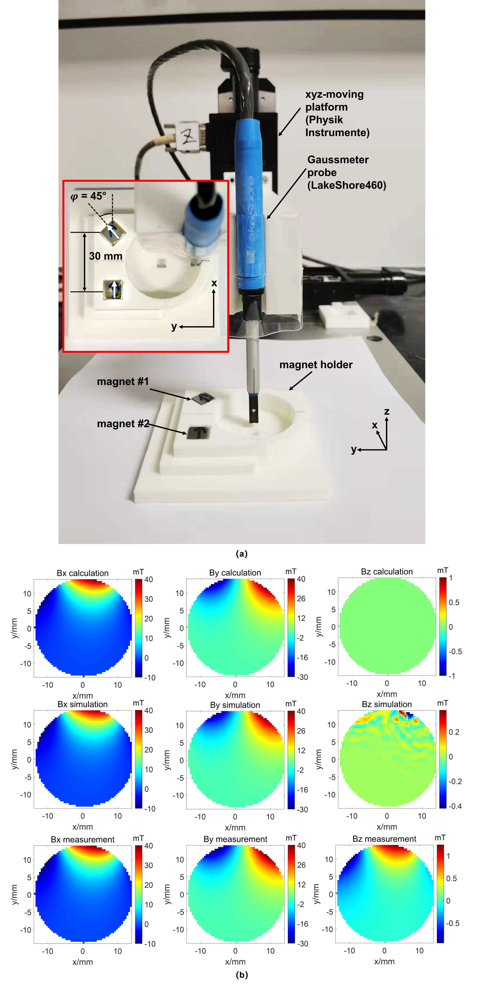
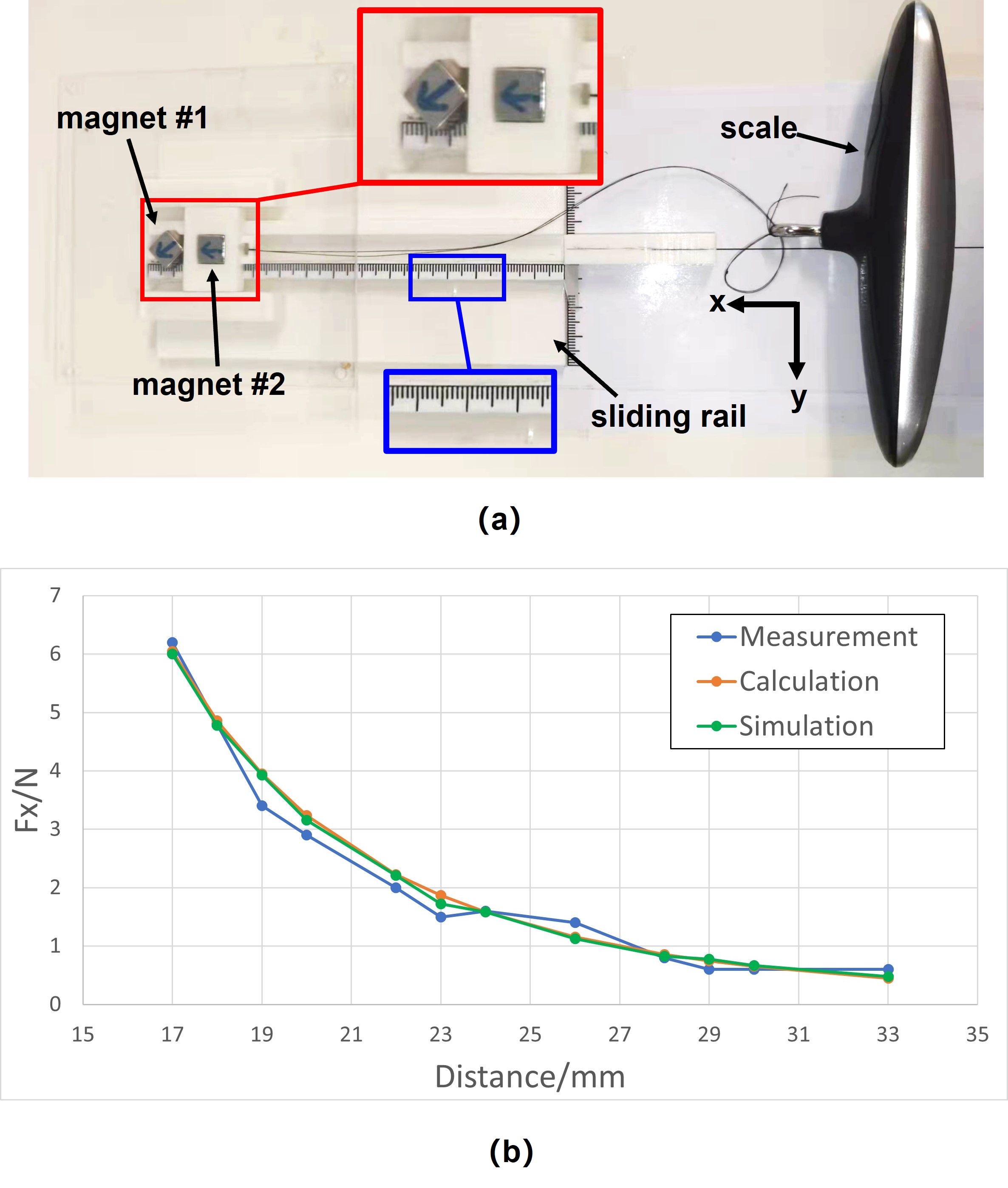
Fig.4(a) shows the 2-magnet setup(10x10x10mm³, $$$B_r$$$=1.40T) for magnetic field measurement, including a Gaussmeter probe (LakeShore460, resolution=0.001mG) fixed on a xyz-moving platform (Physik Instrumente) and a holder for the magnets. The polarization of magnet#1 and #2 are 45° from the x-axis, respectively, 30mm apart in the x-direction. Fig.4(b) shows the comparison of the calculation, CST simulation, and measurement of the x-, y-, and z-field components within a circular FoV (diameter=28mm) on the xy-plane. The maximum discrepancy for the large components($$$B_x$$$, $$$B_y$$$) between the calculation and the simulation is about 6%, and that between the calculation and the measurement is 10%.
Fig.5(a) and (b) show the experiment and the results for the magnetic force measurement of the same 2-magnet setup. The setup consists of a 3D-printed sliding rail (depth=5mm) with magnet#1 fixed at the left end and magnet#2 sliding along the rail. A holder with a thickness of 5mm and a handle was designed to harness the upper half of magnet#2 for pulling for force measurement. 0.5mm of spacing between the rail and magnet#2 is introduced to ensure negligible friction during sliding. Due to the unavailability of high-precision dynamometer at the time, a scale with a resolution of 0.01kg was used for the measurement. The attracting force between the two magnets, $$$F_x$$$, was measured. Fig.4(c) shows the “MagTetris” calculation, CST simulation, and measurement of $$$F_x$$$ at different distances between the two magnets. They match one another closely. The measurement shows an average discrepancy of 4.5% compared to the calculated results, which can be due to the low sensitivity and precision of the scale. For the computational time, it is 7.72s using the FEM-based CST, while it is 0.0628s using “MagTetris”, where “MagTetris” is 123 times faster. The processor used was Intel(R) Core(TM)i7-10750H CPU@ 2.60GHz 2.59GHz.

Conclusion

A magnet simulator, “MagTetris”, is proposed to have a fast calculation of both the magnetic field and force generated by multiple cuboid magnets in arbitrary configurations. It significantly accelerates the calculation speed by 123 times from numerical simulation with uncompromised accuracy. This magnet simulator is a useful tool to support fast permanent magnet array designs and optimizations for various purposes, especially for the recently popular dedicated portable MRI.

Acknowledgements

No acknowledgement found.