4306
Multi-Adaptive Convolutional Neural Network Reconstruction (MA-CNNR) for Parallel Imaging at 1.5T Brain Images1Innovative Technology Laboratory, FUJIFILM Healthcare Corporation, Tokyo, Japan, 2Radiation Diagnostic Systems Division, FUJIFILM Healthcare Corporation, Tokyo, Japan
Synopsis
Recently, deep learning techniques for high-speed or high-quality imaging in MRI have been reported. However, deep learning techniques for the inhomogeneous spatial distribution of noise caused by parallel imaging have not been fully established. In this study, “Multi-Adaptive Convolutional Neural Network Reconstruction (MA-CNNR)” has been investigated. A noisy image was segmented into four regions by g-factor map, and different optimized CNNs were selected for each region. A denoised image was generated by combining the four denoised regions. The denoising effect was evaluated for 1.5T brain images, and it was confirmed that MA-CNNR can reduce the inhomogeneous noise in parallel imaging.
Introduction
Recently, deep learning techniques for high-speed or high-quality imaging in MRI have been reported[1-5]. However, deep learning techniques for the inhomogeneous spatial distribution of noise caused by Parallel Imaging (PI) have not been fully established. In our previous study, “Multi-Adaptive Convolutional Neural Network Reconstruction (MA-CNNR)” has been investigated. It was shown that the inhomogeneous noise can be reduced by segmenting images into two regions and using two types of optimal CNNs for each region in 3T brain images [6]. In this study, we have investigated MA-CNNR and increased the number of segmented regions to reduce the inhomogeneous noise more effectively. The denoising effect was evaluated in 1.5T brain images, and it was found that MA-CNNR can reduce the inhomogeneous noise caused by PI.Method
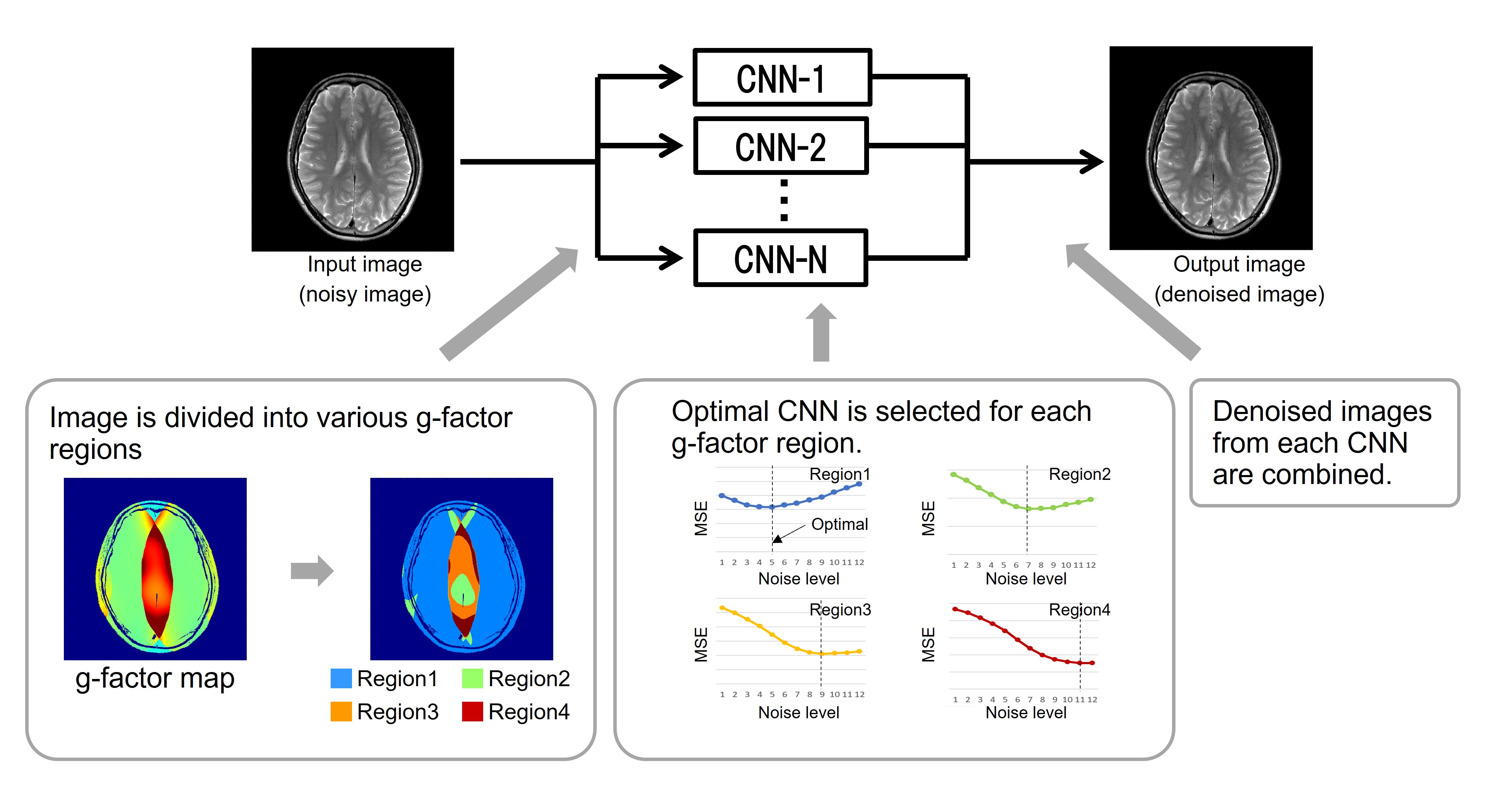
Figure 1 shows a schematic of MA-CNNR. In MA-CNNR, the optimal CNN is selected in accordance with the characteristics of the input image. In this study, a geometry factor (g-factor) map is used for selecting the optimal CNN. In PI, the Signal-to-Noise Ratio (SNR) of images is varied spatially in accordance with the g-factor as below:$$SNR_{PI}(r)=\frac{SNR_{full}(r)}{g(r)\sqrt{R}} $$
where R represents the reduction factor of PI, g represents the geometry factor, and r represents the position. Therefore, we used the g-factor map as noise distribution. In this study, images were segmented into two or four regions in MA-CNNR. In the case of two regions (2-region MA-CNNR), the threshold of the g-factor value was set as 2.0, and in the case of four regions (4-region MA-CNNR), the thresholds were set as 1.5/2.0/2.5. We reduced the noise in N regions by using CNN-1, …, and CNN-N (N=2 or 4). To optimize CNNs, we generated multiple output images denoised by a single CNN trained with a different noise level, and then we optimized noise levels by choosing the CNN that can minimize Mean Square Error (MSE) between the denoised image and full-sampling image for each region. Finally, a denoised image was generated by combining the N regions denoised by CNN-1 to CNN-N. A super-resolution CNN was trained on the dataset[7]. T2 weighted brain images of three volunteers were measured by 1.5T MRI (FUJIFILM Healthcare Corporation). To evaluate the denoising effect, MSE and Structural Similarity Index Measures (SSIM) between the denoised images and full-sampling images were calculated. Second, the denoised image and difference map between the denoised image and full-sampling image were analyzed. This study was approved by the ethics committee of FUJIFILM Healthcare Corporation. All data used in this study were obtained after receipt of written informed consent.
Results
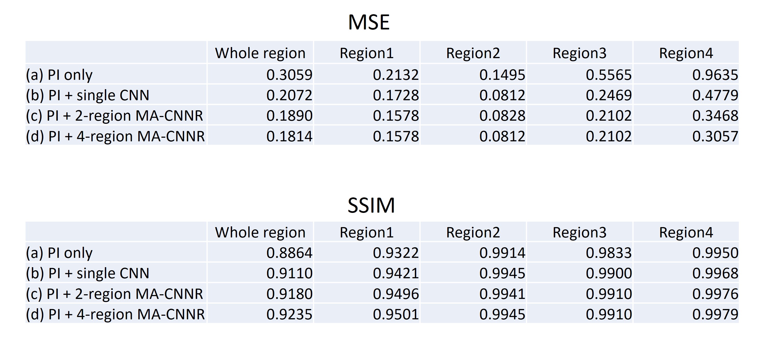
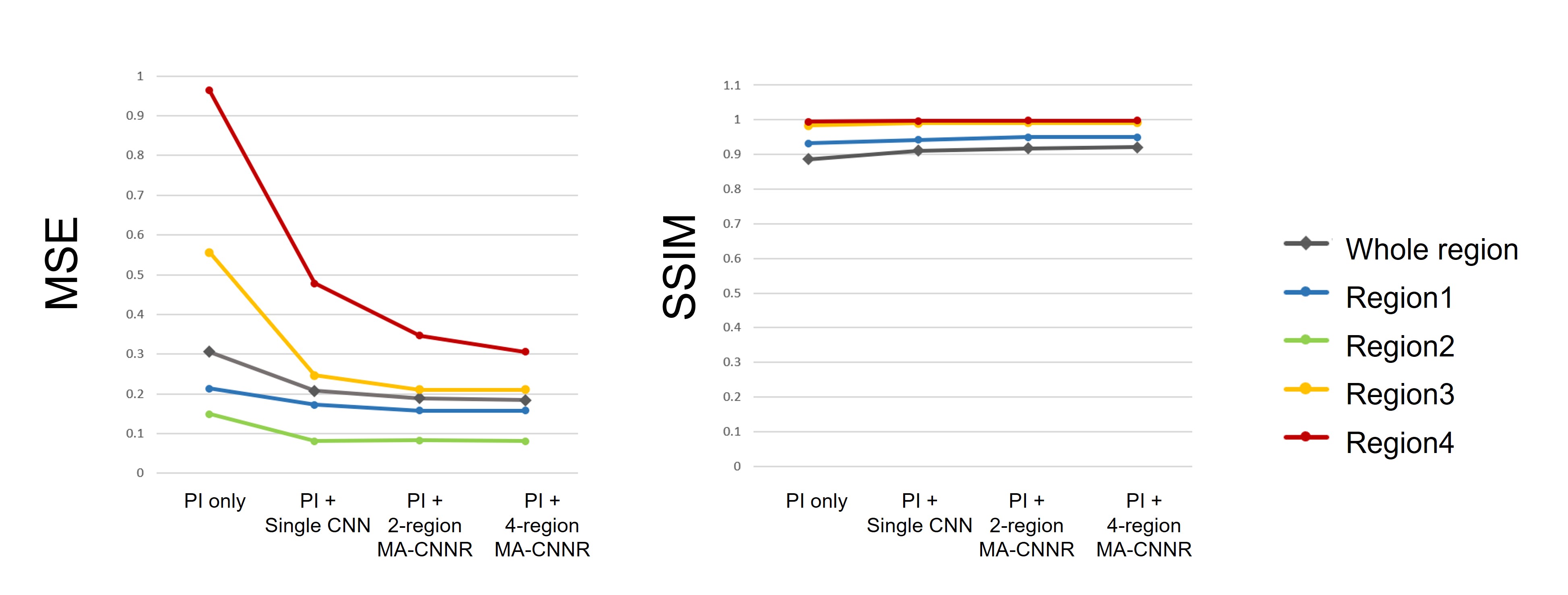
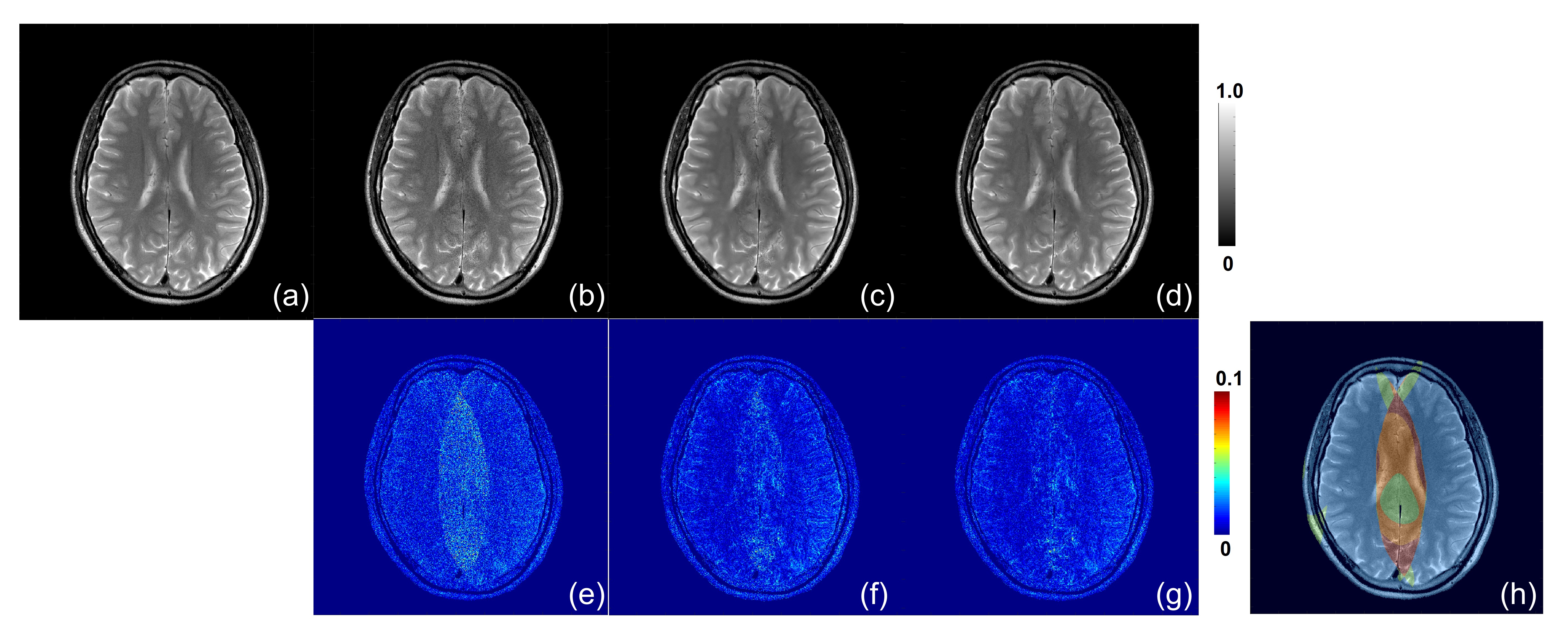
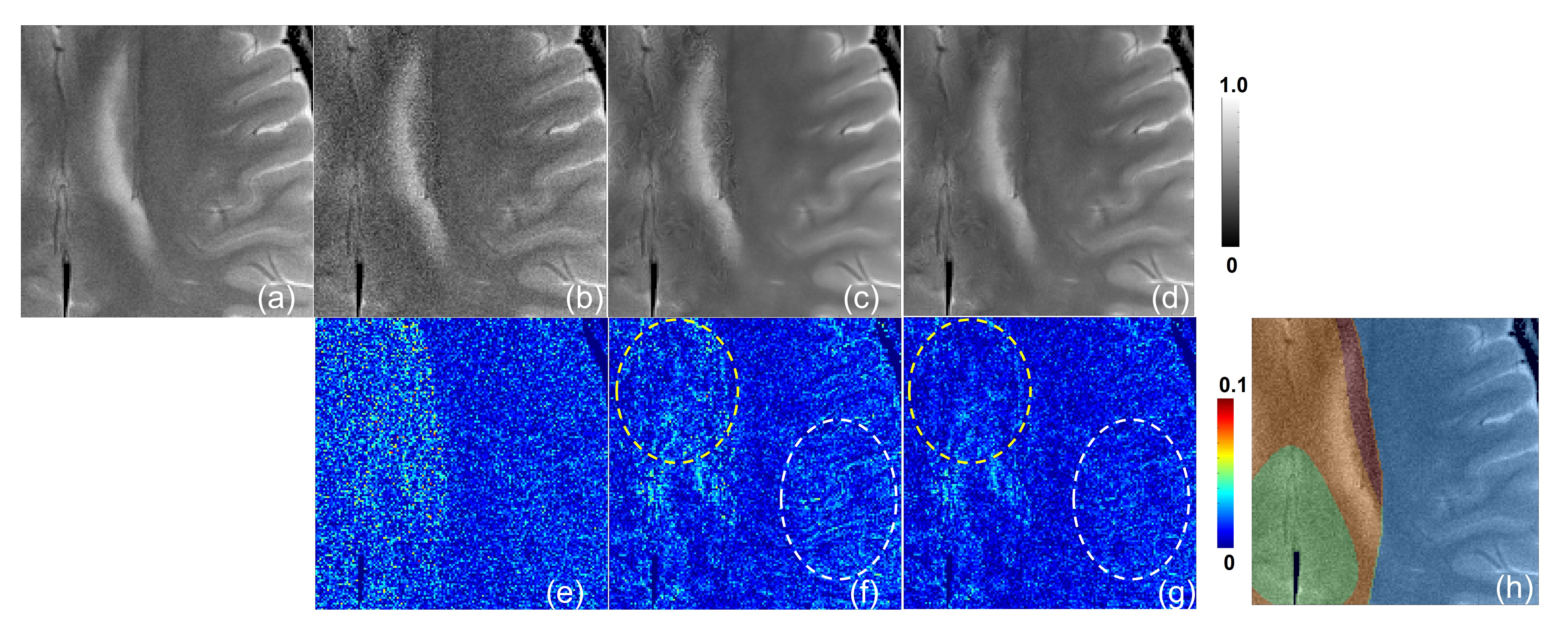
Table1 and Figure 2 show the results of the evaluation index values: MSE and SSIM. 2-region/4-region MA-CNNR (case (c)(d)) have smaller MSEs and larger SSIMs than the conventional single CNN (case (b)). Results show that 4-region MA-CNNR improved MSE and SSIM compared with 2-region MA-CNNR. Figure 3 shows the results of denoised images by using the single CNN and 4-region MA-CNNR. The noise appears in the brain images in PI only (case (b)), and the noise in the central region in the brain image is larger than that in the peripheral region according to the g-factor map. The noise is reduced more by using single CNN and MA-CNNR than PI only. Figure 4 shows the close-ups of the images in Figure 3. In the single CNN (case (c)), the noise in the central region in the image is larger than that in the peripheral region. In the difference map (case (f)), the noise remains in the central region (as shown with yellow circle), and the structure appears in the peripheral region (as shown with white circle). In the difference map (case (g)), the values in the yellow and white region decrease.Discussion
In Table 1 and Fig. 2, 4-region MA-CNNR improved the MSE and SSIM more than 2-region MA-CNNR. In 4-region MA-CNNR, the image was segmented into four regions, and four optimal CNNs were used. It is shown that 4-region MA-CNNR can adjust the inhomogeneous spatial distribution of noise more effectively than 2-region MA-CNNR. In Fig. 4(c) and (f), the noise remains in the central region because the effect of denoising with the single CNN is too weak for this region. On the other hand, the structure appears in the peripheral region because the effect with the single CNN is too strong for this region, and the image was blurred. This indicates that it is difficult to adjust the spatial inhomogeneity of the noise by using the single CNN. MA-CNNR can control the level of denoising for each region by selecting optimal CNN, and has the potential to adjust the inhomogeneous noise caused by PI. Note that the acceleration factor was 3 (scan time was 1/3) in this study. However, MA-CNNR can be applied to images with a higher acceleration factor.Conclusion
In this study, we investigated MA-CNNR and increased the number of segmented regions to reduce the inhomogeneous noise more effectively. The denoising effect was evaluated for 1.5T brain images, and it was found that MA-CNNR can reduce the inhomogeneous noise by PI.Acknowledgements
No acknowledgement found.References
1. Lin DJ, Johnson PM, Knoll F, et al. Artificial Intelligence for MR Image Reconstruction: An Overview for Clinicians. J Magn Reson Imaging. 2020; 53(4):1015-1028.
2. Jiang D, Dou W, Vosters L, et al. Denoising of 3D magnetic resonance images with multi-channel residual learning of convolutional neural network. Jpn J Radiol. 2018; 36: 566–574.
3. Kawamura M, Tamada D, Funayama S, et al. Accelerated Acquisition of High-resolution Diffusion-weighted Imaging of the Brain with a Multi-shot Echo-planar Sequence: Deep-Learning-based Denoising. Magn Reson Med Sci. 2020; 20(1):99-105.
4. Rao G Sasibhushana, Srinivas B. De-Noising of MRI Brain Tumor Image using Deep Convolutional Neural Network. Proc. of International Conference on Sustainable Computing in Science, Technology and Management (SUSCOM). 2019.
5. Kidoh M, Shinoda K, Kitajima M, et al. Deep Learning Based Noise Reduction for Brain MR Imaging: Tests on Phantoms and Healthy Volunteers. Magn Reson Med Sci. 2020; 19 (3):195-206.
6. Suzuki A, Ishihara C, Kaneko Y, et al. Deep-learning-based Noise Reduction Incorporating Inhomogeneous Spatial Distribution of Noise in Parallel MRI Imaging, Proc. of ISMRM 2021; 29: 3264.
7. Dong C, Loy C, He K, et al. Image Super-Resolution Using Deep Convolutional Networks. IEEE Transactions on Pattern Analysis and Machine Intelligence. 2016; 38 (2): 295-307.
Figures