4305
B1- and B1+ based bias field correction for ultra-high field MRI
Yi-Cheng Hsu1, Patrick Liebig2, and Ying-Hua Chu1
1Siemens Healthineers Ltd., Shanghai, China, 2Siemens Healthcare GmbH, Erlangen, Germany
1Siemens Healthineers Ltd., Shanghai, China, 2Siemens Healthcare GmbH, Erlangen, Germany
Synopsis
We proposed a method to approximate the magnitude of B1- and correct the bias field induced signal inhomogeneity at 7T. For 2D and 3D T2 weighted images, the signal intensity was more homogeneous and the signal void was recovered using the proposed method. This method can be implemented to correct bias field effect for other imaging methods using the estimated |B1-| and |B1+|.
Introduction
B1 inhomogeneity is one of the main problems that limit the clinical application of ultra-high-field MRI. The spatially varying contrast and intensity influence diagnosis and need to be corrected. For magnetic resonance imaging at fields lower than, or equal to 3 T, B1 shimming technology can provide more uniform B1+, which is sufficient for clinical application. By comparing the signal intensity of coil arrays with the flat receive profile of a volume coil, we can estimate B1- and correct for this non-uniform intensity distribution. At the ultra-high field, the B1 inhomogeneity is more severe and both above-mentioned methods are inadequate. Parallel transmission (pTx)1 can excite a more uniform flip angle by accelerated spatially selective excitation. However, this method required special hardware and minor flip angle inhomogeneity together with B1- effect still exists after pTx excitation. The most widespread post-processing methods for B1+ and B1- correction are nonparametric nonuniform intensity normalization (N3)2, and its' improved version, N4ITK3. However, the assumption, the effect of bias field (the combining effect of B1+ and B1-) can be approximate as a convolution of Gaussian function to the distribution of the true tissue intensity, is not applicable when the bias field is strong. To overcome these difficulties, we estimated the magnitude of B1- and proposed a bias-field correction method based on its signal dependence on B1- and B1+.Methods
For a spoiled gradient echo sequence at low flip-angle, the signal can be approximated as:$$PD(r)=M_0 (r)⋅\alpha⋅|B_1^+ (r)|⋅|B_1^- (r)|⋅f(T1(r),T2(r),TE,TR)$$
, where f is the function of T1 and T2 relaxation and α is the nominal flip angle. We need the information of M0, |B1+| and $$$f(T1(r),T2(r),TE,TR)$$$ to estimate |B1-|. For brain imaging, low flip angle proton density weighted images usually present low tissue contrast ($$$M_0⋅f(T1(r),T2(r),TE,TR)\approx Constant$$$), and can be used to estimate $$$|B_1^-(r)|$$$ when $$$|B_1^+ (r)|$$$ is available.
Therefore, we approximated the bias field in the brain based on the proton density images:
$$B_1^±(r)=C⋅|B_1^+ (r)|⋅|B_1^- (r)|=Sfilter(PD(r))$$
,where Sfilter is an operator that approximates the images using multi-resolution 3D splines3.
For an imaging method, named MET, its signal can be expressed as:
$$I_{MET}(r)=|B_1^- (r)|⋅g_{MET}(T1(r),T2(r),α⋅|B_1^+ (r)|)⋅M_0(r)$$
,where gMET is a method-dependent function that describes its signal dependence on T1, T2 and B1+. With the information of $$$B_1^±(r)$$$ and $$$|B_1^+(r)|⋅$$$ The bias field corrected images can be calculated as:
$$I_{METcor}(r)=I_{MET}(r)/\frac{B_1^±(r)}{|B_1^+(r)|}/g_{MET}(T1(r),T2(r),\alpha⋅|B_1^+ (r)|).$$
In most situations as well as in this study, T1 and T2 maps are not available. Therefore, we approximated T1 and T2 by constants, $$$\bar{T1}$$$ and $$$\bar{T2}$$$. The PD-weighted images were acquired with parameters (TE/TR=2.41/20ms, flip angle=5o, FOV=220x220x220mm3, and matrix size=80x80x80). The |B1+| maps were acquired using pre-saturation TFL (FOV=220x220x220mm3, matrix size=64x64x30). We acquired 3D SPACE T2 weighted images (TE/TR=118/4000ms, ETL=119,FOV=212x150x170mm3, and matrix size=318x224x256) and 2D TSE T2 weighted images (TE/TR=54/320ms, ETL=11, FOV=209x209x72 mm3, matrix size=1176x1568x30, and slice thickness=2mm) to test the performance of the proposed method. The function gMET for both methods were calculated based on phase graph theory4. One healthy volunteer was scanned at a 7T MRI system (MAGNETOM Terra, Siemens Healthineers, Erlangen, Germany).
Results
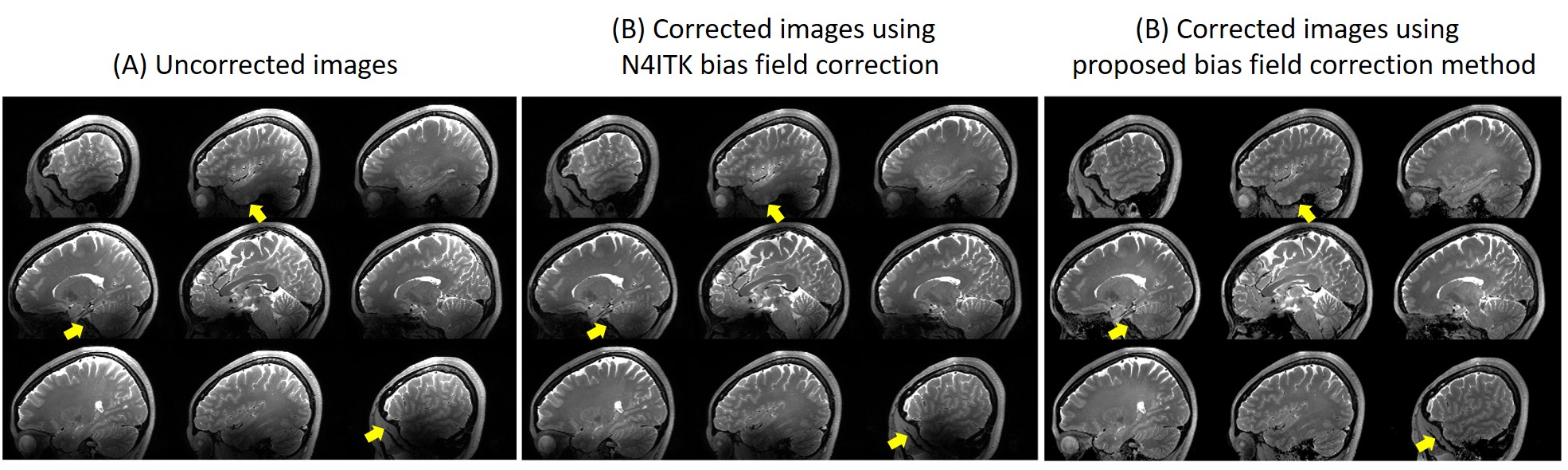
Figure 1A shows the PD-weighted images. The $$$B_1^±$$$ maps estimated from the PD-weighted images were shown in Figure 1B, and |B1+| maps at the same slices were shown in Figure 1C. Figure 2A shows SPACE T2 weighted images at the same slices of Figure 1B without bias field correction. The bias field caused signal voids near the temporal lobe and inferior part of the cerebellum. Figure 2B are the images after N4ITK bias field correction. For most brain regions, the signal inhomogeneity was improved, however, it fails in regions of low B1. Figure 2C shows the images using the proposed bias field correction. The image intensity is more homogeneous and the signal voids in the temporal lobe and cerebellum were recovered.Figure 3A shows the T2 TSE images of the healthy volunteer. The image homogeneity, using the proposed post-processing method, improves significantly in figure 3B. There were more structural details that can be seen in the temporal lobe and inferior cerebellum.
Discussion and Conclusion
We proposed a method to estimate a B1- map. Together with the measured B1+ map, we were able to correct the image intensity inhomogeneity caused by the bias field. This method can be applied to correct bias field effects for different imaging protocols or sequences using the same estimated bias field maps. On the contrary, for most post-processing methods, the bias field was estimated from the targeted images3,5 and these estimation might be inaccurate if the targeted images only have limited coverage.The signal intensity depends not only on the bias field but also on its T1 and T2 properties. Note that the proposed method cannot correct the contrast altered by the bias field. The pTx is a better solution to achieve homogeneous contrast by a more uniform excitation. However, the proposed method can be used to correct the B1- inhomogeneity and the residual flip angle inhomogeneity in images using pTx.
In most situations, we don't need extra proton density images. For example, we can use the magnitude images from field mapping with the least echo time, or the unsaturated images used for TFL B1 mapping and thereby not adding additional scan time.
Acknowledgements
No acknowledgement found.References
- Katscher, Ulrich, et al. Transmit sense. Magnetic Resonance in Medicine 49.1 (2003): 144-150.
- Sled, John G., Alex P. Zijdenbos, and Alan C. Evans. A nonparametric method for automatic correction of intensity nonuniformity in MRI data. IEEE transactions on medical imaging 17.1 (1998): 87-97.
- Tustison, Nicholas J., et al. N4ITK: Improved N3 Bias Correction.”IEEE Transactions on Medical Imaging 29.6 (2010): 1310–20.
- Weigel, M., et al. Extended phase graphs with anisotropic diffusion. Journal of magnetic resonance 205 (2010): 276–285.
- Chebrolu, Venkata Veerendranadh, et al. Uniform Combined Reconstruction (UNICORN) of Multi-Channel Surface-Coil Data at 7T without Use of a Reference Scan. ISMRM 2018: 3524.
Figures
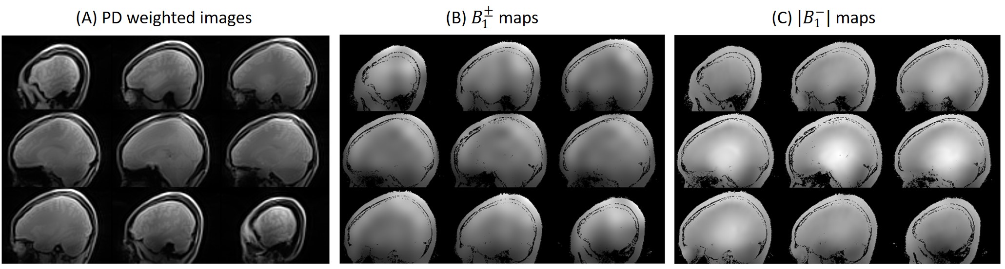
Figure 1. (A) Nine slices of the proton density images used to estimate |B1-|. (B) Nine slices of the estimated B1± that was resliced to match the resolution and location of 3D T2 images (Figure 2). (C) Nice slices of the estimated |B1+| that was resliced to match the resolution and location of 3D T2 images.
Figure
2. (A) Nine slices of the acquired 3D T2 weighted images. (B) The 3D T2
weighted images after N4ITK bias field correction. (C) The 3D T2 weighted
images post-processed by the proposed bias field correction method.
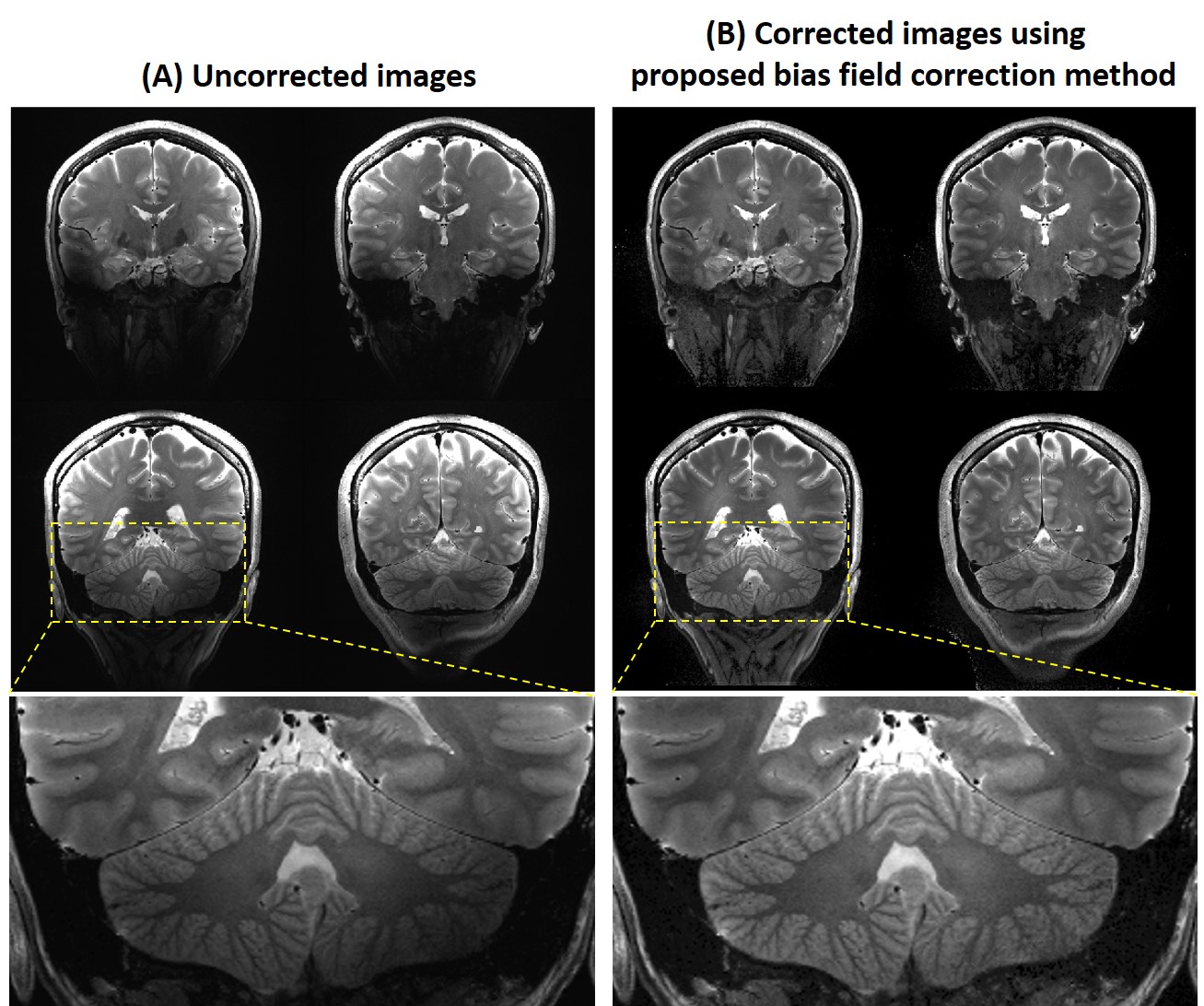
Figure 3. (A) Four slices of the acquired 2D T2
weighted images. (B) The 2D T2 weighted images post-processed by the proposed
bias field correction method.
DOI: https://doi.org/10.58530/2022/4305