Introduction

Cardiac cine MRI is important for clinical examination and evaluation of cardiovascular diseases since it can present the shape, motor function, and myocardial activity of the heart. However, the artifacts caused by breathing and heartbeat are a challenge in cardiac MR imaging. Although the commonly used under-sampling strategy speeds up the data acquisition, it also causes artifacts in the image domain. Therefore, fast data acquisition and high-quality image reconstruction are vital for dynamic MRI, which can capture both anatomical and temporal information.
High-resolution acquisition approaches in k-space and super-resolution approaches after reconstruction in the image domain have been reported [1-3]. These methods either have limited performance at certain high acceleration factors or suffer from the error accumulation of a two-step structure. In order to preserve the important details, we propose a multi-scale detail preserving reconstruction method for dynamic MR image reconstruction. Specifically, the residuals of multi-scale intermediate images in the iterative procedure are explored and the temporal and spatial dependencies between frames are considered. We employ multi-scale super-resolution and bidirectional convLSTM as the sparse regularization term in each reconstruction step to explore its prior knowledge. This method can refine image details that are neglected by existing methods, and achieve superior visual and quantified performance at high acceleration factors, such as 11.

Method

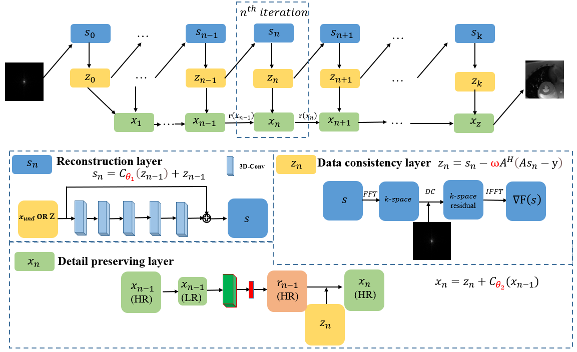
The proposed method targets high-quality image reconstruction at high acceleration factors. The overall architecture is shown in Figure 1. The details are described as follows. Eq. 1 summarizes the CS-MRI model for MR reconstruction, which is an inverse problem. It can be solved as an unconstrained optimization problem (Eq. 2) and different types of prior knowledge can be exploited through the regularization term $$$R(x)$$$. Two auxiliary variable $$$s$$$ and $$$z$$$ are introduced, where $$$z$$$ is constrained to be equal to $$$x$$$ and $$$s$$$ is constrained to be equal to $$$z$$$. Then, we can reconstruct $$$x$$$ by minimizing Eq. 3, and Eq. 3 can be solved via minimizing three sub-problems shown in Eq. 4. Finally, the iterative procedures given in Eq. 5 are utilized to optimize the three sub-problems.
$$y=Ax+e\quad\quad\quad\quad\quad (1)$$
$$arg\min_x⁡R(x)+ \frac{1}{2}‖Ax-y‖_2^2\quad\quad\quad\quad (2)$$
$$arg\min_x\frac{1}{2}‖Ax-y‖_2^2+R(s)+δ‖s-z‖_2^2+ε‖z-x‖_2^2\quad\quad\quad\quad (3)$$
\begin{cases}\displaystyle s_n=arg\min_sδ‖s-z_{n-1}‖_2^2+R(s)\quad\quad\quad\quad\quad\quad\quad\quad\quad\quad (4a)\\\displaystyle z_n=arg\min_z⁡δ‖z-s_n‖_2^2+∇F(s_n)\quad\quad\quad\quad\quad\quad\quad\quad\quad\quad (4b) \\\displaystyle x_n=arg\min_s\frac{α}{2}‖Ax-y‖_2^2+ε‖x-z_n‖_2^2+r(x_n )\quad\quad\quad\quad (4c) \\\end{cases}
\begin{cases}s_n=Prox(z_{n-1})\quad\quad\quad\quad\quad\quad\quad\quad (5a)\\z_n=s_n-ωA^H (As_n-y)\quad\quad\quad\quad\quad (5b)\\x_n=z_n+∆x_n\quad\quad\quad\quad\quad\quad\quad\quad\quad (5c)\\\end{cases}
In Eq. 1, $$$x∈\mathbb{C}^N$$$ represents 2D cardiac high-quality sequences, $$$A∈\mathbb{C}^{M×N}$$$ is the under-sampling operator, $$$y∈\mathbb{C}^M (M≪N)$$$ is the under-sampled k-space data, and $$$e∈\mathbb{C}^M$$$ is the noise term. In Eq. 2, ⁡$$$R(x)$$$ represents the regularization of $$$x$$$, $$$\frac{1}{2}‖Ax-y‖_2^2$$$ is data fidelity term, and $$$δ$$$ and $$$ε$$$ are two penalty parameters. In Eq. 3, $$$R(s)$$$ represents the regularization of $$$s$$$. In Eq. 4, we define $$$F(x)$$$ as the data fidelity term $$$\frac{1}{2}‖Ax-y‖_2^2$$$, and we can update $$$z_n$$$ from $$$s_n$$$ by minimizing $$$F(x)$$$. Since $$$z_n$$$ is a linear combination of $$$s_n$$$ and the original measurement $$$y$$$, we can transfer Eq. 4b to minimize $$$‖z-s_n‖_2^2$$$ and the correction term $$$∇F(s_n)$$$. In order to update $$$x_n$$$ from $$$z_n$$$, we expect the reconstruction values in iteration steps $$$n$$$ and $$$n-1$$$ to be equal by introducing a correction term $$$r(x_n )$$$ between $$$x_n$$$ and $$$x_{n-1}$$$.
We unroll the iterations into a deep neural network. The three procedures in Eq. 5 correspond to three modules in the network as shown in Fig. 1. They are named as the reconstruction layer $$$s_n$$$, the data consistency layer $$$z_n$$$, and the details preserving layer $$$x_n$$$. All parameters $$$(θ_1,ω,θ_2)$$$ in Eq. 6-8 are learnable network parameters.
\begin{cases}s_n=C_{θ_1}(z_{n-1})+z_{n-1}\quad\quad\quad\quad\quad (6)\\z_n=s_n-ωA^H(As_n-y)\quad\quad\quad\quad (7)\\x_n=z_n+C_{θ_2} (x_{n-1})\quad\quad\quad\quad\quad\quad (8)\\\end{cases}
where $$$C_{θ_1}$$$ represents the five 3D convolution layers in the reconstruction module and $$$θ_1$$$ refers to the learnable parameters. $$$ω$$$ is the update step size in the data consistency modules. $$$x_n$$$ consists of two parts. One is a cascade of seven 2D convolution layers and the ReLU activation function. The other is bidirectional convLSTM between $$$ x_n$$$ and $$$x_{n-1}$$$. $$$θ_2$$$ represents the learnable parameters in $$$C_{θ_2}$$$ .

Experimental configurations

T1-weighted FLASH sequence is utilized to collect fully sampled cardiac data from 101 volunteers on a 3T scanner. Each scan acquires a single slice from the volunteer with 25 temporal frames. After data augmentation, our dataset consists of 5634 complex-valued cardiac MR data. For each frame, we employ a shear grid k-t Cartesian sampling pattern with an acceleration factor of 11 to undersample the k-space data to generate the undersampled input image sequences. For reconstruction results, we compare our approach with some existing cardiac reconstruction algorithms under the same acceleration factor, including the CNN-based deep cascade reconstruction method (D5C5) [4] and the multi-supervised training model in k-space and image domain (DIMENSION) [5].

Result

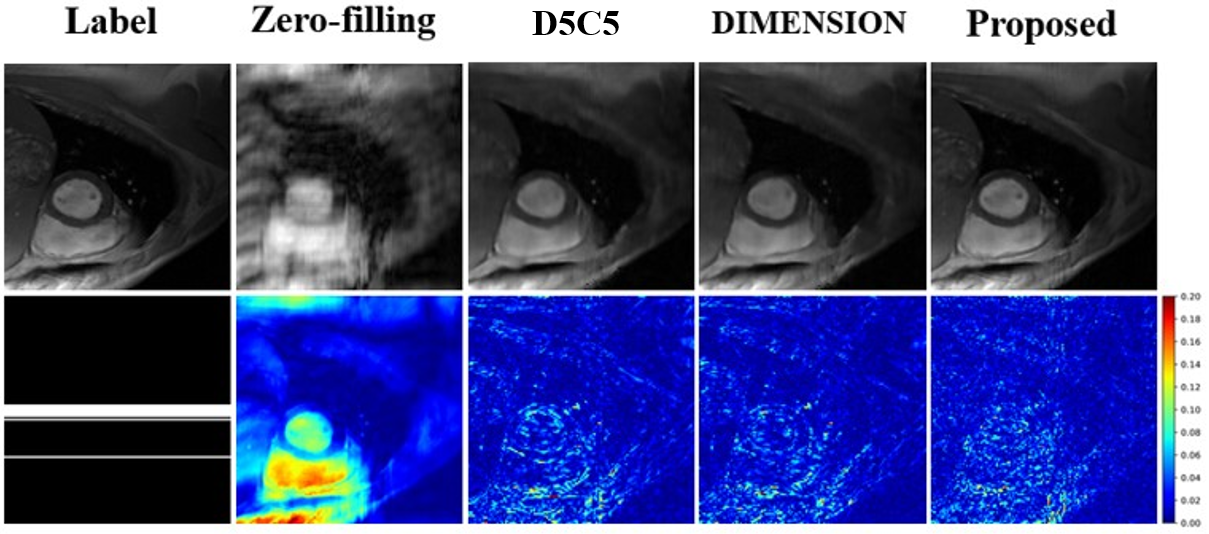
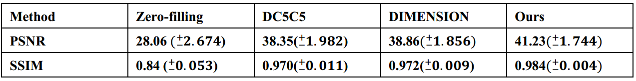
Table 1 lists the quantitative results. Compared with existing methods, our method generates better reconstruction results characterized by PSNR and SSIM. Figure 2 shows some qualitative reconstruction results. From these qualitative results, we observe that our method can reconstruct images with smaller errors and are better at detail preservation and artifact removal when compared to the other two recent methods.

Conclusion

In this study, we propose a multi-scale detail-preserving reconstruction method for dynamic MRI, which employs multi-scale super-resolution and bidirectional convLSTM as the sparse regularization term in each reconstruction step. Experimental results show that our method achieves better reconstruction results both quantitatively and qualitatively compared to two state-of-the-art image reconstruction methods.

Acknowledgements

This research was partly supported by Scientific and Technical Innovation 2030-"New Generation Artificial Intelligence" Project (2020AAA0104100, 2020AAA0104105), and the National Natural Science Foundation of China (61871371, 81830056)