4086
MR thermometry using fingerprinting: application to lead heating
Enlin Qian1, Pavan Poojar1, David H. Gultekin1, J. Thomas Vaughan1, Devashish Shrivastava1, Zhezhen Jin2, Brett E. Youngerman3, and Sairam Geethanath1
1Columbia Magnetic Resonance Research Center, Columbia University, New York, NY, United States, 2Department of Biostatistics, Columbia University, New York, NY, United States, 3Columbia University Irving Medical Center, Columbia University, New York, NY, United States
1Columbia Magnetic Resonance Research Center, Columbia University, New York, NY, United States, 2Department of Biostatistics, Columbia University, New York, NY, United States, 3Columbia University Irving Medical Center, Columbia University, New York, NY, United States
Synopsis
We explore the feasibility of noninvasive temperature measurement around deep brain stimulation (DBS) leads using magnetic resonance fingerprinting (MRF) by leveraging 1) the dependency of T1 on temperature; 2) MRF’s efficient T1 and B0 mapping. We conducted a T1 and temperature calibration experiment and a lead calorimetry experiment on bovine muscle. The effects of B0 inhomogeneity and temperature profiles of different regions of interest (ROI) were investigated. The calibration showed a strong correlation between temperature and T1 (R2>0.98). We observed a maximum change of 10.2 oC near leads (~1mm away) during calorimetry experiments, validated by fluoroptic probes.
Introduction
MR thermometry provides noninvasive temperature measurements in near real-time 1. After implantation of DBS leads, magnetic resonance imaging (MRI) may be clinically necessary. However, heating induced near lead electrodes during MRI remains a safety concern 2. An MR thermometry scout may enable heat monitoring and introduce cooling periods to keep heating below a safe threshold and ensure safety.In this work, we demonstrate the feasibility of using MRF for temperature measurements near DBS lead by exploiting T1 relaxation time’s dependence on temperature while simultaneously estimating B0 map.
Method
MRF implementationThe MRF sequence uses parameters reported in previous literature 4, 5. The acquisition time was 18 seconds/slice. Data were reconstructed using singular value decomposition (SVD) dictionary matching 6. The reconstruction time was ~30 seconds/slice.
Calibration experiment
Figure 1(a) shows the setup for calibration experiment. We ran MRF sequence every 5 minutes after experiment started. Fluoroptic probes measured temperatures every second. The experiment lasted 125 minutes.
Four ROIs with 60 voxels were selected based on the position of probes (Figure 2(a)). The mean T1 of each ROI was calculated. The corresponding probes’ temperatures were averaged over MRF acquisition (18 seconds). Simple linear regression and R2 statistics were calculated using least-squares fitting.
Lead experiment
Figure 1(b) shows the setup for lead experiment. We ran MRF sequence first to measure baseline temperature, followed by a 16:26 (min:s) turbo spin-echo (TSE) sequence to induce heating. After the heating, we ran MRF protocol every minute for 10 minutes to measure temperature as it returned to baseline. Fluoroptic probes measured temperatures every second. We repeated the cycle three times and acquired a TSE structure image for ROI selection. The experiment lasted 75 minutes.
One ROI with 60 voxels was selected 1 mm away from the tip of the lead. The maximum value of ROI was calculated. The corresponding probes’ temperatures were averaged over MRF acquisition.
B0 experiment
Due to orientation limitations for gold standard B0 maps acquisition, we conducted a separate experiment to investigate the effects of B0 inhomogeneity around lead. The lead was inserted into the cold bovine muscle, same as lead experiment. A vendor sequence (fast GRE-based B0 mapping) with TR=250 ms and FA=30o was run to acquire gold standard B0 maps. The acquisition time was 2:12 (min:s). We then ran MRF sequence to compare B0 maps.
Spatial temperature gradient analysis
We selected ROIs 1 mm, 3 mm, and 6 mm away from the tip of lead electrode to investigate the spatial temperature gradients near the lead.
Results/Discussion
Figure 2(a) shows that T1 decreases as the heated bovine muscle cooled down for the first 30 minutes of the experiment. The T1 of the room temperature water bottle serves as a reference and stays ~2 seconds for entire experiment. The cold muscle has longer T1 than heated muscle because the heated muscle loses water during heating process which we drained. Figure 2(b) presents the best fit line for the center of cold muscle and center and periphery of heated muscle and their respective R2 statistics. All R2 values are larger than 0.988, indicating a strong linear relationship between temperature and T1. This linear relationship agrees with previous literature 1, 7.Figure 3(a) and (b) show the T1 and temperature map of the first cycle in the lead experiment. T1 increases as temperature increases due to TSE-induced heating. The heating was more evident around the lead. An ROI was selected in (c) to investigate the temperature estimated by MRF and temperature measured by fluoroptic probes. (d) shows that MRF estimated temperature has a similar trend as probe temperature, but the range is smaller compared to the probe temperatures. This may be because the ROI was 1 mm away from the tip of the lead and the spatio-temporal averaging of the T1 caused the ROI to experience less amount heating as the probe.
Figure 4 shows that the B0 map estimated using MRF had similar regions of inhomogeneity but underestimated gold standard B0 map. The gold standard B0 map showed ~200 Hz inhomogeneity around lead area, while the MRF estimated ~150 Hz. Figure 4(b) presents joint T1 and B0 mapping. The figures show that more signal was recovered resulting in a longer T1. This may have a significant impact on accurate estimation of temperature near lead because of the inhomogeneity generated by lead electrodes.
Figure 5 shows the positions of three different ROIs that are 1 mm, 3 mm, and 6 mm from the tip of the lead and their maximum values for each time point respectively. The 1 mm ROI has the largest temperature change (~ 10 degrees) and the 6 mm ROI has the smallest temperature change (~ 4 degrees), similar to findings in 2. The starting temperatures for ROIs were different because the temperature of the muscle was not homogeneous when the experiment started.
Conclusion
We investigated the feasibility of measuring temperature near DBS lead using MRF based T1 and B0 mapping. T1 and temperature show strong correlation (R2 > 0.988). We observed a maximum change of 10.2 oC near leads during calorimetry experiments, validated by fluoroptic probes. The effects of B0 and distance from the lead were investigated.Acknowledgements
This work was supported, in part, by GE-Columbia research partnership grant and also performed at Zuckerman Mind Brain Behavior Institute MRI Platform, a shared resource, and Columbia MR Research Center site. The subject matter, content, and views presented do not represent the views of the Department of Health and Human Services (HHS), US Food and Drug Administration (FDA), and/or the United States.References
- Rieke V: MR Thermometry. In Interventional Magnetic Resonance Imaging. Edited by Kahn T, Busse H. Berlin, Heidelberg: Springer Berlin Heidelberg; 2012:271–288.
- Shrivastava D, Abosch A, Hughes J, et al.: Heating induced near deep brain stimulation lead electrodes during magnetic resonance imaging with a 3 T transceive volume head coil. Phys Med Biol 2012; 57:5651–5665.
- Ma D, Gulani V, Seiberlich N, et al.: Magnetic resonance fingerprinting. Nature 2013; 495:187–192.
- Jiang, Y., Ma, D., Seiberlich, N., Gulani, V., & Griswold, M. A. (2015). MR fingerprinting using fast imaging with steady state precession (FISP) with spiral readout. Magnetic Resonance in Medicine. https://doi.org/10.1002/mrm.25559
- Shridhar Konar A, Qian E, Geethanath S, et al.: Quantitative imaging metrics derived from magnetic resonance fingerprinting using ISMRM/NIST MRI system phantom: An international multicenter repeatability and reproducibility study. Med Phys 2021.
- McGivney DF, Pierre E, Ma D, et al.: SVD compression for magnetic resonance fingerprinting in the time domain. IEEE Trans Med Imaging 2014; 33:2311–2322.
- Nelson TR, Tung SM: Temperature dependence of proton relaxation times in vitro. Magn Reson Imaging 1987; 5:189–199.
Figures
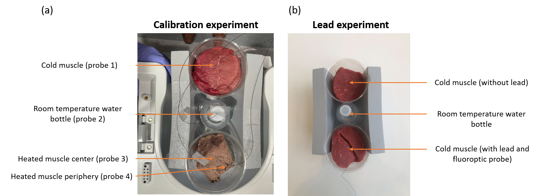
Figure 1. Experimental Setup Figure 1 shows the setup for (a) calibration experiment and (b) lead experiment. Calibration experiment consists of cold bovine muscle, room temperature water bottle for reference, and heated bovine muscle. Four fluoroptic probes were inserted into the center of cold bovine muscle, the water bottle, and center and periphery of heated muscle. The lead experiment consisted of cold bovine muscle with and without lead and a room temperature water bottle. We attached the fluoroptic probe at the tip of the lead with tape and inserted it into the cold bovine muscle.
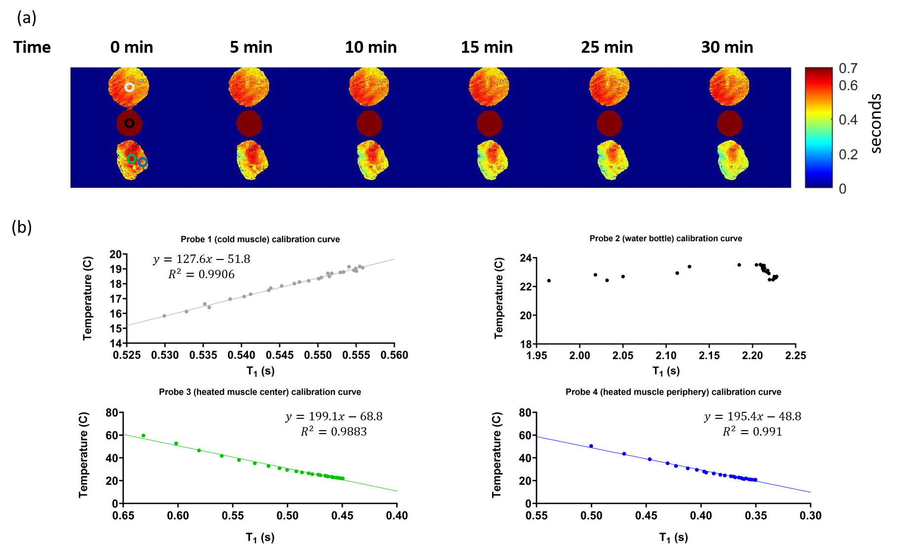
Figure 2. Calibration (a) A series of T1 maps acquired using MRF at first 30 minutes with 5 minutes intervals during calibration experiment. The time represents the total time from beginning of the experiment. ROIs were drawn based on probes locations to calculate T1 around the probes. (b) The mean of T1 calculated using ROIs over the measured fluoroptic probe temperatures for all probes and the resulting linear relationship using least square fitting. The linear regression lines and corresponding R2 values are presented. No fitting was performed for the room temperature water bottle.
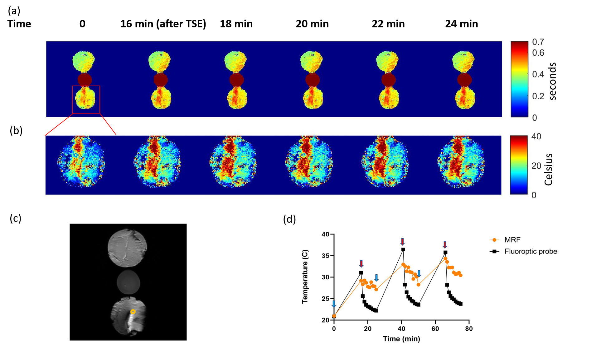
Figure 3. Lead heating Figure 3 shows (a) the first cycle of T1 maps acquired using MRF during lead experiment. The time represents the total time from beginning of the experiment. (b) A series of magnified temperature maps of muscle with lead corresponding to T1 maps in (a) using the calibration equation. (c) A structure image acquired using TSE. We selected ROI 1 mm away from the tip of the lead. (d) The comparison of temperature estimated using MRF and probe temperature. The baselines for each cycle are marked with blue arrows. The measurements after TSE heating are marked with red arrows.
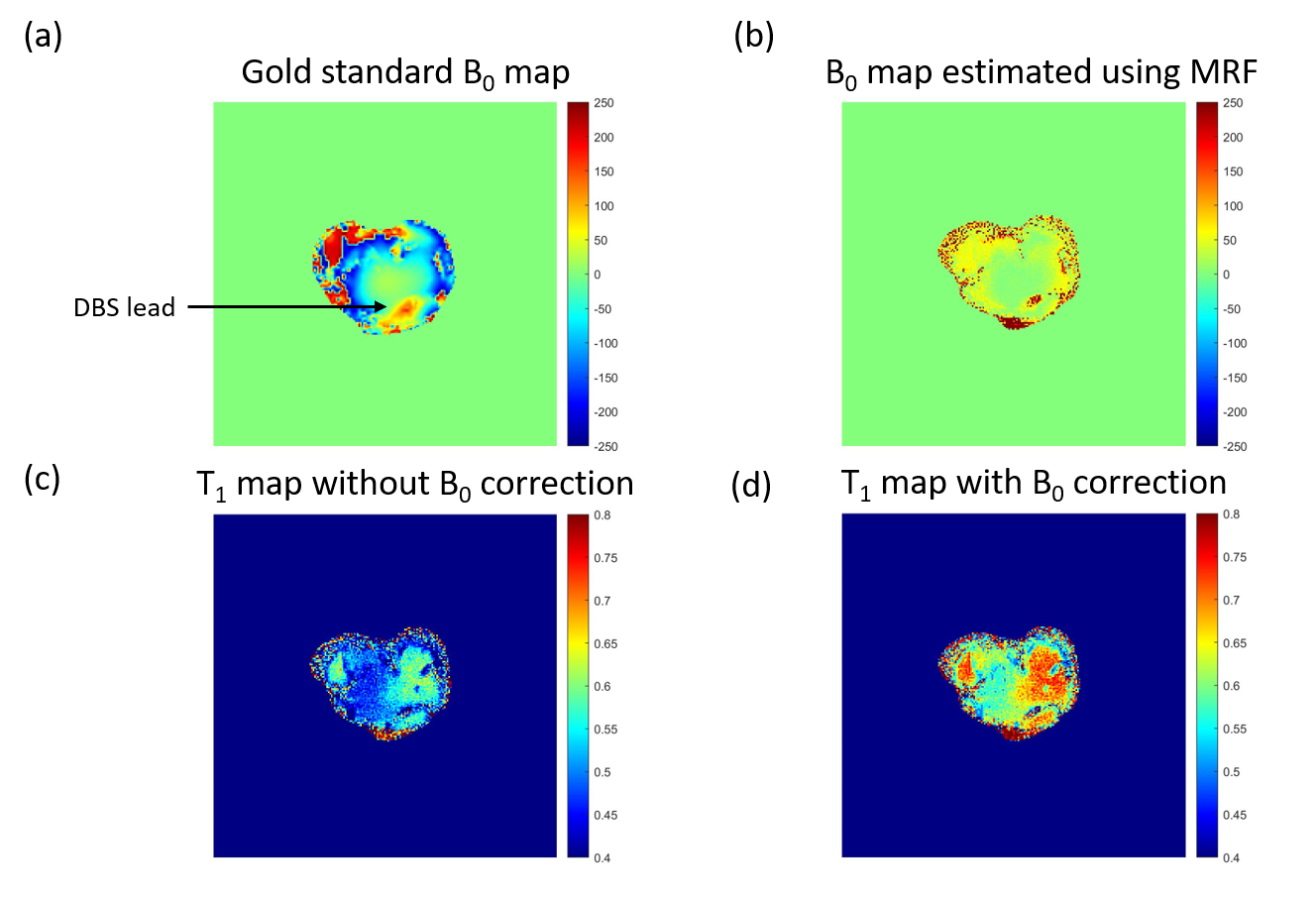
Figure 4. Joint B0 mapping Figure 4 shows our separate experiment investigating the effects of B0 inhomogeneities on the lead and T1 maps. The lead was inserted from the bottom of the muscle and its position is marked with the black arrow. (a) shows the gold standard B0 map acquired using a vendor fast GRE sequence (b) shows the B0 map estimated using MRF. (c) shows the resulting T1 map estimated using MRF with and (d) without B0 correction.
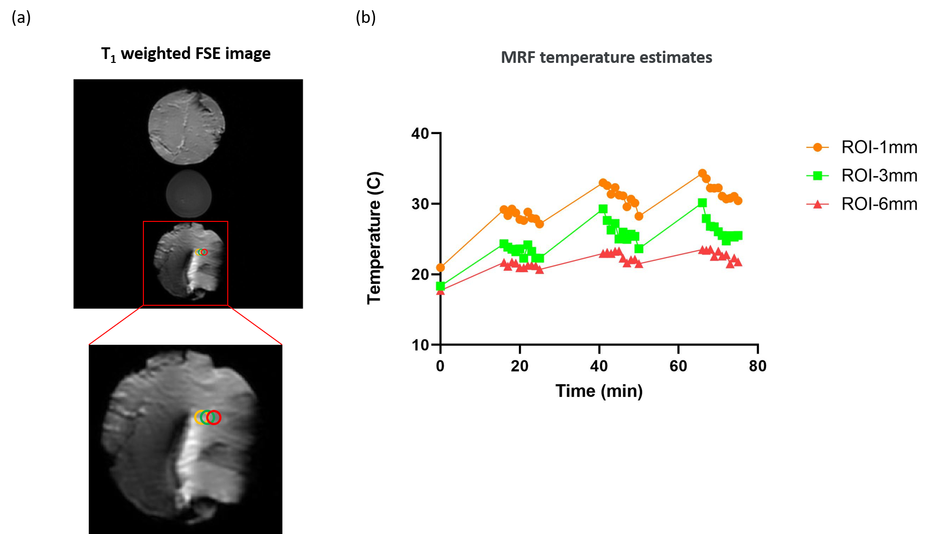
Figure 5. Spatial temperature gradient Figure 5 presents three ROIs with 1 mm, 3 mm, and 6 mm distance (corresponding to 1 voxel, 3 voxels, and 6 voxels) to the lead. Each ROI contains 60 pixels. (a) shows the position of these three ROIs on the T1 weighted structure image acquired using TSE. The image below is the magnified region of the ROIs. (b) shows the maximum temperature of the ROIs for each time point estimated using MRF and the calibration equation.
DOI: https://doi.org/10.58530/2022/4086