4076
Initial Evaluation of a Transverse Isotropic Finite Difference Model for Training Learned Inversion1Mayo Clinic, Rochester, MN, United States
Synopsis
While most existing inversion algorithms used in MR elastography assume that the mechanical properties of tissue are isotropic, many tissues exhibit spatial anisotropy in structure that is not accommodated by these algorithms.1,2 In this work we present a framework for developing a learned inversion to address transverse isotropy, the simplest anisotropic case. A transversely isotropic stiffness matrix was used in a feed forward finite difference model to generate simulated displacements. The squared wave speeds anisotropic inclusions were calculated using direct inversion to validate the model against the theoretical wave speeds.3
Introduction
Magnetic resonance elastography is a non-invasive imaging technique for measuring tissue stiffness akin to manual palpation.4 Traditionally, most inversion algorithms used in the field, which estimate mechanical properties from the measured displacement field, assume isotropic mechanical properties.5,6,7,8 However, in tissues that have anisotropic structure, like muscle or white matter tracts in the brain, mechanical anisotropy, if not negligible, may yield biased results using these algorithms.9 For this reason, several groups are now investigating approaches to anisotropic inversion using both analytical and iterative approaches.10 Learned inversions,2 which can be conceptualized as unrolled iterative algorithms,11,12 can be adapted to this problem with an appropriate forward model to generate training data. Therefore, the goal of this study was to implement a finite difference model of wave motion in transversely isotropic materials and validate the results against known analytical solutions to the wave equations.Method
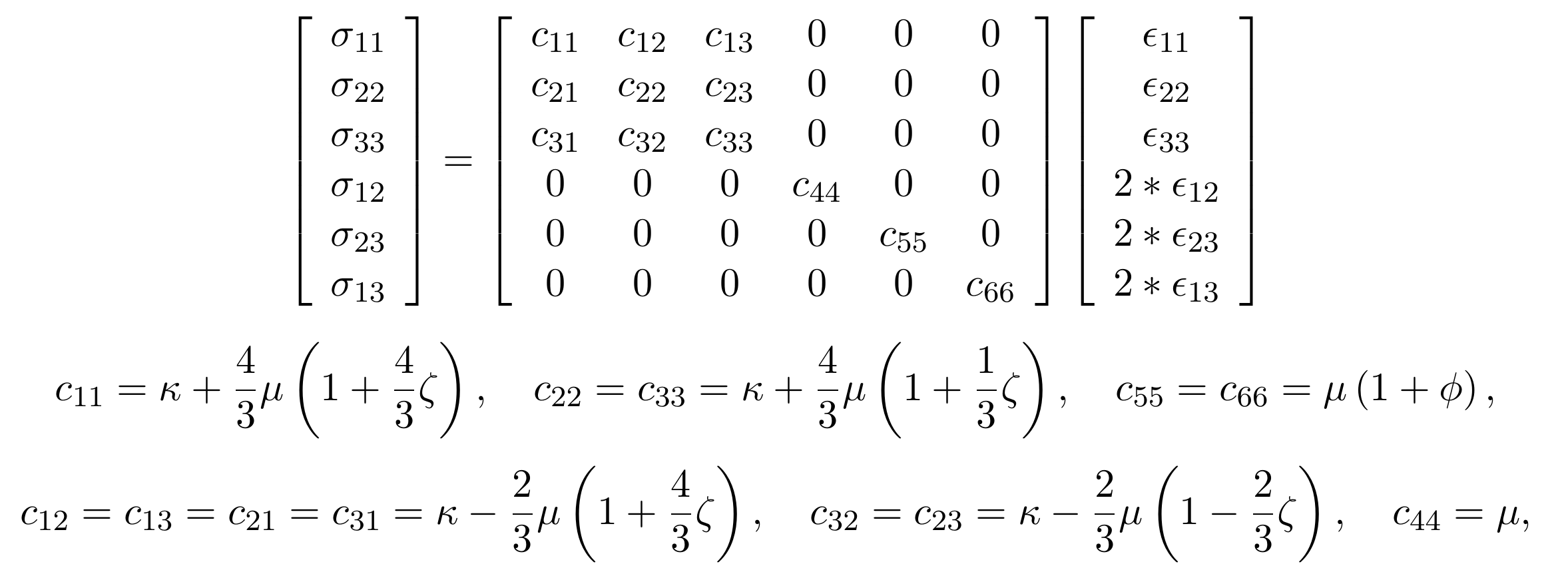
FDM SetupThe wave equation for harmonic motion in an elastic material is given by $$$\nabla\cdot\sigma=\frac{\partial^2 u}{\partial t^2}$$$, where $$$u$$$ is the displacement field and $$$\sigma$$$ is the stress field. For Hookean materials under small strain, this wave equation can be approximated as a linear system according to:
$$-D^TR^TCRED(u+ub)=-\rho\omega^2*I(u+ub)$$
where $$$u$$$ are the displacements to be estimated, $$$ub$$$ are the boundary conditions that induce motion, $$$\rho$$$ is density, $$$\omega$$$ is angular frequency, $$$D$$$ is the gradient operator, $$$E$$$ is a strain operator, $$$R$$$ rotates the strains into the material reference frame, and $$$C$$$ is the stiffness matrix. This system can be rearranged into an overdetermined linear system, $$$Au = f$$$, whose least squares solution is given by $$$u = (A*A)^{-1}A*f$$$, where $$$*$$$ denotes the adjoint of an operator. After parameterizing the material properties, material coordinates, and boundary conditions, we solved this system for each simulation using conjugate gradient method, stopping after 10,000 iterations.
Validation Experiments
For a transversely isotropic material, the stiffness matrix is governed by 5 independent parameters. In this study we parameterized those values according to previously defined formulas,3,14 so that the closed form solutions described could be used for validation.
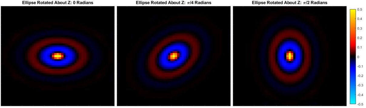
First, simulated examples were made to confirm wave propagation conformed to the expected anisotropic directions. A cubic region with shear anisotropy of 1 and tensile anisotropy of 1 was created using the stiffness formulation in equations 1. This results in anisotropy in the $$$x$$$ direction. A simple case was devised in which a rod placed in the center of the volume, along the $$$z$$$ direction induces motion in the $$$z$$$ direction. As expected, the resulting shape of the displacements appears as an ellipse (Fig 1). To confirm rotation was working as expected, the fiber direction was rotated at $$$\pi/4$$$ and $$$\pi/2$$$ radians about the $$$z$$$-axis. As expected, the long axis of the ellipse was rotated $$$\pi/4$$$ and $$$\pi/2$$$ radians, respectively.
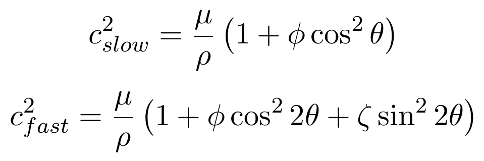
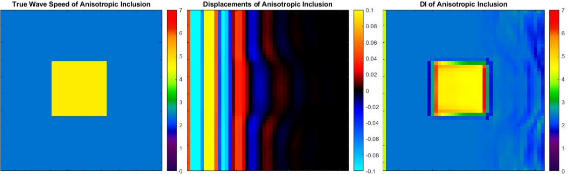
To validate the implementation, simulated examples were made to confirm that calculated wave speeds match the known theoretical values for fast and slow waves (Equation 2).3 Simulations were of a cubic volume with free boundary conditions except on the left face where planar shear waves were introduced with particle motion in the $$$z$$$-direction and propagation in the $$$x$$$-direction. The volume contained isotropic material with an inclusion of an anisotropic rectangular prism which extends along the $$$z$$$-axis, giving a cross sectional image of a square (Fig 2). The prism’s fiber direction was in the $$$x$$$ direction when no rotation was prescribed. Direct inversion (DI) was used to calculate the wave speed inside the anisotropic inclusion and in the isotropic volume (Fig 2). Medians of each region were taken to compare against the theoretical slow wave and fast wave speeds.
In the case of the anisotropy rotating around the $$$z$$$-axis the expected result is for the DI wave speed in the anisotropic cube to match the theoretical slow wave speed described in equation 2. For this rotation, the shear anisotropy, $$$\phi$$$, was $$$1$$$ and tensile anisotropy, $$$\zeta$$$, was $$$0$$$. When the anisotropy is rotating around the $$$y$$$ axis, the expected result is for the wave speed in the anisotropic inclusion to match the fast wave speed described in equation 2. For this rotation, shear anisotropy, $$$\phi$$$, was $$$0$$$ and tensile anisotropy, $$$\zeta$$$, was $$$1$$$. For each axis of rotation, the angle was varied from $$$0$$$ to $$$\pi/2$$$ uniformly in 16 steps.
Results
The model produces the expected ellipse case for each example rotation (Fig 1). Simulations of an anisotropic inclusion in an isotropic volume are invertible with DI following curl calculation and return the correct wave speeds for both the isotropic background and the anisotropic inclusion (Fig 2). The median values of the simulated wave speeds correspond to the theoretical values in cases of both slow wave dominance and fast wave dominance (Fig 3).Conclusion
The anisotropic finite difference model, as it has been implemented, accurately produces wave forms for anisotropic inclusions dominated by both the fast wave regime and the slow wave regime. Furthermore, the framework built to handle rotations of the shear stresses and strains allows for the arbitrary choice of direction of transverse isotropy. This model provides a basis for creating locally transverse isotropic volumes for the training of learned anisotropic inversions.Acknowledgements
Research reported in this publication was supported by the National Institute of Biomedical Imaging and Bioengineering of the National Institutes of Health under award numbers EB001981, EB027064.References
[1] A. Manduca, V. Dutt, D. T. Borup, R. Muthupillai, J. F. Greenleaf, and R. L. Ehman, “Inverse approach to the calculation of elasticity maps for magnetic resonance elastography,” in Medical Imaging 1998: Image Processing, Jun. 1998, vol. 3338, pp. 426–436. doi: 10.1117/12.310921.
[2] J. M. Scott et al., “Artificial neural networks for magnetic resonance elastography stiffness estimation in inhomogeneous materials,” Medical Image Analysis, vol. 63, p. 101710, Jul. 2020, doi: 10.1016/j.media.2020.101710.
[3] D. J. Tweten, R. J. Okamoto, J. L. Schmidt, J. R. Garbow, and P. V. Bayly, “Estimation of material parameters from slow and fast shear waves in an incompressible, transversely isotropic material,” J Biomech, vol. 48, no. 15, pp. 4002–4009, Nov. 2015, doi: 10.1016/j.jbiomech.2015.09.009.
[4] R. Muthupillai and R. L. Ehman, “Magnetic resonance elastography,” Nat Med, vol. 2, no. 5, pp. 601–603, May 1996, doi: 10.1038/nm0596-601.
[5] A. J. Romano, J. J. Shirron, and J. A. Bucaro, “On the noninvasive determination of material parameters from a knowledge of elastic displacements theory and numerical simulation,” IEEE Transactions on Ultrasonics, Ferroelectrics, and Frequency Control, vol. 45, no. 3, pp. 751–759, May 1998, doi: 10.1109/58.677725.
[6] T. E. Oliphant, A. Manduca, A. Dresner, R. Ehman, and J. Greenleaf, “Adaptive Estimation of Piece-wise Constant Shear Modulus for Magnetic Resonance Elastography,” p. 1.
[7] E. e. w. Van Houten, K. d. Paulsen, M. i. Miga, F. e. Kennedy, and J. b. Weaver, “An overlapping subzone technique for MR-based elastic property reconstruction,” Magnetic Resonance in Medicine, vol. 42, no. 4, pp. 779–786, 1999, doi: 10.1002/(SICI)1522-2594(199910)42:4<779::AID-MRM21>3.0.CO;2-Z.
[8] S. Papazoglou, U. Hamhaber, J. Braun, and I. Sack, “Algebraic Helmholtz inversion in planar magnetic resonance elastography,” Phys. Med. Biol., vol. 53, no. 12, pp. 3147–3158, May 2008, doi: 10.1088/0031-9155/53/12/005.
[9]A. T. Anderson et al., “Observation of direction-dependent mechanical properties in the human brain with multi-excitation MR elastography,” J Mech Behav Biomed Mater, vol. 59, pp. 538–546, Jun. 2016, doi: 10.1016/j.jmbbm.2016.03.005.
[10] M. M. Doyley, P. M. Meaney, and J. C. Bamber, “Evaluation of an iterative reconstruction method for quantitative elastography,” Phys. Med. Biol., vol. 45, no. 6, pp. 1521–1540, May 2000, doi: 10.1088/0031-9155/45/6/309.
[11] R. Miller, A. Kolipaka, M. P. Nash, and A. A. Young, “Estimation of transversely isotropic material properties from magnetic resonance elastography using the optimised virtual fields method,” International Journal for Numerical Methods in Biomedical Engineering, vol. 34, no. 6, p. e2979, 2018, doi: 10.1002/cnm.2979.
[12] Hammernik, K. et al. Learning a variational network for reconstruction of accelerated MRI data. Magnetic resonance in medicine 79, 3055-3071 (2018).
[13] Monga, V., Li, Y. & Eldar, Y. C. Algorithm unrolling: Interpretable, efficient deep learning for signal and image processing. IEEE Signal Processing Magazine 38, 18-44 (2021).
[14] M. McGarry et al., “A heterogenous, time harmonic, nearly incompressible transverse isotropic finite element brain simulation platform for MR elastography,” Physics in Medicine and Biology, vol. 66, p. 055029, Mar. 2021, doi: 10.1088/1361-6560/ab9a84.
Figures