4072
Simulation of a Virtual Liver Iron-overload Model and Estimation of R2* Using Complex Fat-Water Models1Biomedical Engineering, The University of Memphis, Memphis, TN, United States
Synopsis
Multi-spectral fat-water-R2* modeling techniques fit either a single R2* or estimate independent R2* for water and fat molecules. In this study, a virtual liver model with hepatic iron overload was created based on true histological data and MRI signals were synthesized using Monte Carlo simulations. Our results demonstrate that the dual R2* values predicted by the ARMA model exhibit relaxivity behavior similar to in vivo and thus can be used for R2* estimation in vivo in varying concentrations of iron overload.
Introduction
Multi-spectral fat-water-R2* modeling techniques like non-linear square (NLSQ) fitting and autoregressive moving average (ARMA) have been proposed for the quantification of R2* and fat fraction (FF)1,2. The NLSQ model assumes a single R2* for both fat and water peaks to avoid model complexity. While on the other hand, the ARMA model estimates independent R2* for water and fat protons. Inaccurate assumptions in calculating R2* values can cause error in R2* estimation leading to clinical misdiagnosis. The main purpose of this study is to develop a virtual liver model with varying hepatic iron concentrations (HICs) that accurately mimics a realistic human liver and synthesize MRI signals using Monte Carlo simulations3,4 to compare the accuracy of single and dual R2* values with in-vivo R2*-HIC calibration5,6.Methods
Ghugre et. al developed a Monte-Carlo model for R2*-iron calibration based on published statistics of hepatic iron scale and distribution and magnetic properties3,4,7. This Monte-Carlo model was reproduced by constructing 80*80*80 µm³ virtual iron overload liver models with varying HICs based on gamma distribution function. Susceptibility value of 1.6 E-6 m3/kgFe was chosen equivalent to the 4:1 mixture of human hemosiderin and ferritin and expected magnetic field inhomogeneities induced by the iron deposits were modeled using:$$\triangle B(r,\theta)=B_0/3*\chi*(R/r)^3*(3cos^2\theta-1)$$
where, B0 is the applied magnetic field (1.5T), χ is the particle susceptibility, R is the sphere radius, r is the radial distance between the center of the iron sphere and proton position, and θ is the azimuthal angle to the magnetic axis.
5000 protons were randomly distributed across the liver volume at a magnetic strength of 1.5T and allowed to do a random walk for 10ms. Their mobility was characterized as Brownian motion using:
$$\sigma=\sqrt{2*D*\delta}$$
where, D = 0.76µm2/ms is the diffusion coefficient8 and 𝛿=0.5µs is the proton time step.
The phase accrual ϕ for each proton at the end of each time step t was calculated using:
$$\phi (t)=\gamma \delta \sum_{i=1}^{t} (B_0+\triangle B(p(i)))$$
where, γ=2.675*108 rads-1T-1 is the gyromagnetic ratio, p(i) is the ith proton position.
Superposition of phase accrual of the protons as they pass through the induced magnetic disturbances will produce the synthetic MRI signals with different relaxation rates depending on varying HICs.
The signal from each proton was calculated as:
$$ S(t)=S(0)e^{(-t*R2_0+j\phi (t))}$$
where, S(0) is signal amplitude at t=0 and R20 is the relaxation in normal liver. The superposition of signals from all protons yields the total synthesized signal.
All Monte Carlo simulations were performed using Python and relaxivities were then calculated using multi-spectral fat-water ARMA and NLSQ models. NLSQ model was implemented from the ISMRM Fat-Water Toolbox9,10 and ARMA model was implemented as an iterative approach with a maximum of 7 peaks1. A one-way ANOVA was done on Sigma Plot to compare the slopes of R2*-HIC regression lines of the multi-spectral fat-water and monoexponential models with Wood et al. R2*-biopsy HIC calibration5.
Results and Discussion
Virtual liver models mimicking published human histological statistics were simulated for different iron concentrations ranging from 2.5-25 milligrams per gram of dry weight of liver (Figure 1). Synthesized MRI signals exhibited faster signal decays with increasing values of HIC (Figure 2). Predicted dual R2* values exhibited positive correlation with HIC values, with slopes similar to in vivo R2*-HIC calibration and fell within 95% predicted confidence interval of Wood et al. R2*-HIC calibration (Figure 3, Table 1). The single R2*-HIC values also showed positive correlation with in-vivo R2*-HIC calibration and fell within 95% predicted confidence interval. However, the NLSQ model displayed inconsistent values of fat fractions for HIC values above 20 mg Fe/g tissue. The monoexponential model showed a perfect correlation with Wood’s calibration. The slopes of the regression lines for all models did not show significant difference (p-value: 0.831) compared to Wood calibration. The multi spectral fat-water models, however, seemed to be influenced by even slight oscillations in the signal decay towards the later echoes. These oscillations have caused the FWT model to give false fat fractions, but this needs further investigation.Conclusion
Our results demonstrates that ARMA exhibits positive correlation with in vivo R2*-HIC calibration. So, our study suggests that ARMA can be used for quantification of iron in liver.Future work includes simulating MRI signals in higher magnetic strengths, and with a greater number of protons for higher signal to noise ratio and using a truncated approach to reduce the effects of oscillations in the signals in case of high iron concentrations. Future work also involves simulating liver models in coexisting conditions of iron overload and steatosis.
Acknowledgements
Grant support: Supported by grant 1R21EB031298 from the National Institute of Health.
References
1. Tipirneni-Sajja A, Krafft AJ, Loeffler RB, et al. Autoregressive moving average modeling for hepatic iron quantification in the presence of fat. J Magn Reson Imaging. 2019;50(5):1620-1632. doi:10.1002/jmri.26682
2. Hernando D, Liang ZP, Kellman P. Chemical shift-based water/fat separation: a comparison of signal models. Magn Reson Med. 2010;64(3):811-822. doi:10.1002/mrm.22455
3. Ghugre NR, Gonzalez-Gomez I, Shimada H, Coates TD, Wood JC. Quantitative analysis and modelling of hepatic iron stores using stereology and spatial statistics. J Microsc. 2010;238(3):265-274. doi:10.1111/j.1365-2818.2009.03355.x
4. Ghugre NR, Wood JC. Relaxivity-iron calibration in hepatic iron overload: probing underlying biophysical mechanisms using a Monte Carlo model. Magn Reson Med. 2011;65(3):837-847. doi:10.1002/mrm.22657
5. Wood JC, Enriquez C, Ghugre N, et al. MRI R2 and R2* mapping accurately estimates hepatic iron concentration in transfusion-dependent thalassemia and sickle cell disease patients. Blood. 2005;106(4):1460-1465. doi:10.1182/blood-2004-10-3982
6. Hankins JS, McCarville MB, Loeffler RB, et al. R2* magnetic resonance imaging of the liver in patients with iron overload. Blood. 2009;113(20):4853-4855. doi:10.1182/blood-2008-12-191643
7. Ghugre NR, Gonzalez-Gomez I, Butensky E, et al. Patterns of hepatic iron distribution in patients with chronically transfused thalassemia and sickle cell disease. Am J Hematol. 2009;84(8):480-483. doi:10.1002/ajh.21456
8. Yamada I, Aung W, Himeno Y, Nakagawa T, Shibuya H. Diffusion coefficients in abdominal organs and hepatic lesions: evaluation with intravoxel incoherent motion echo-planar MR imaging. Radiology. 1999;210(3):617-623. doi:10.1148/radiology.210.3.r99fe17617
9. Hernando D, Kellman P, Haldar JP, Liang ZP. Robust water/fat separation in the presence of large field inhomogeneities using a graph cut algorithm. Magn Reson Med. 2010;63(1):79-90. doi:10.1002/mrm.22177
10. Hu HH, Börnert P, Hernando D, et al. ISMRM workshop on fat-water separation: insights, applications and progress in MRI. Magn Reson Med. 2012;68(2):378-388. doi:10.1002/mrm.24369
Figures

Figure 1. Virtual iron overload model with volume 80 µm * 80 µm *80 µm and a representative HIC of 15 mg / g, and the corresponding 2D slice of dimension 80 µm * 80 µm and thickness 5 µm.
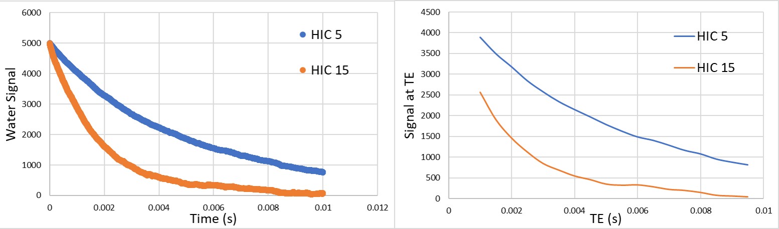

Figure 3. Linear regression analysis between HIC and predicted R2* obtained from single and dual R2* multi-spectral fat-water models and monoexponential model with published in vivo R2*-HIC calibrations. The dashed line indicates 95% predicted interval of Wood’s regression line.

Table 1. Slopes, y-intercepts, and R-squared values of the regression equations obtained from regression analysis in Figure 3.