4047
Practical Approaches to the Evaluation of Signal-to-Noise Ratio Performance with Deep Learning Denoising Image Reconstruction1Biomedical Engineering, University of Wisconsin-Madison, Madison, WI, United States, 2Radiology, University of Wisconsin-Madison, Madison, WI, United States, 3Medical Physics, University of Wisconsin-Madison, Madison, WI, United States, 4Medicine, University of Wisconsin-Madison, Madison, WI, United States, 5Emergency Medicine, University of Wisconsin-Madison, Madison, WI, United States
Synopsis
In this work, three methods for measuring signal-to-noise ratio (SNR) performance of deep learning (DL) denoising image reconstruction were evaluated. Images reconstructed using a vendor prototype DL reconstruction algorithm were compared to conventional Fourier reconstruction. Phantom experiments were performed using a single-channel head coil and a 32-channel head coil to assess the effects of parallel imaging acceleration in combination with DL reconstruction on SNR performance. We found excellent agreement between the three SNR measurement methods for both Fourier and DL reconstruction, and found that DL reconstructed images have similar g-factor performance patterns as Fourier reconstructed images.
Introduction
Deep learning (DL) has led to multiple applications in MR image reconstruction, including denoising algorithms. While it has been shown that the application of DL image reconstruction can be used to boost apparent SNR1, there are no standard approaches to quantify the SNR performance of DL reconstruction algorithms. Therefore, the purpose of this work is to evaluate practical methods to quantify SNR from MR images reconstructed using a DL algorithm.Theory
MR signal noise has a Gaussian distribution with zero mean2. Conventionally, the SNR of a pixel within a complex-valued image is measured as the ratio of average signal magnitude ($$$S$$$) to the standard deviation of noise ($$$\sigma$$$), ie:\begin{equation}SNR=\frac{S}{\sigma}\tag{1}\end{equation}Conventional Method
In Fourier reconstructed images without parallel imaging acceleration, the noise is evenly distributed after Fourier transformation. With this assumption, SNR can be measured as the ratio of the average signal in a region of interest (ROI) inside the object to the standard deviation of the noise in an ROI outside the object. For magnitude reconstructed images, measured SNR must be corrected by a constant factor, $$$\alpha$$$, due to the presence of rectified noise3,4.\begin{equation}SNR=\alpha\frac{S}{\sigma}\tag{2}\end{equation}
Multiple-Acquisition Method
The complexity of DL reconstruction algorithms adds to the uncertainty of noise distribution (e.g., spatial invariance) in the reconstructed images. Therefore, other methods to evaluate SNR are needed. One method to quantify SNR is to acquire images under identical conditions multiple times, where SNR can be determined on a pixel-by-pixel basis: \begin{equation}SNR=\frac{\bar{S}}{\sigma_s}\tag{3}\end{equation}
For each pixel, $$$\bar{S}$$$ refers to the average signal, and $$$\sigma_s$$$ the standard deviation, over multiple images. This method does not require the assumption of spatial invariance of noise.
Difference Method
A third approach5 is to estimate SNR from two identically acquired images $$$S_1$$$ and $$$S_2$$$, where the mean of the signal and the standard deviation of the signal are obtained from the same ROI with assumption of uniform signal and noise within the ROI, but not necessarily across the image. \begin{equation}SNR_{ROI}=\frac{S_{ROI}}{\sigma_{ROI}}=\frac{mean(S_1+S_2)\vert_{ROI}}{\sqrt{2}std(S_1-S_2)\vert_{ROI}}\tag{4}\end{equation}
Parallel Imaging and g-factor
With parallel imaging, there is spatially dependent noise amplification characterized by g-factor5, 6, ie:
\begin{equation}g(R)=\frac{SNR_0}{\sqrt{R}SNR_R}\tag{5}\end{equation}
For each pixel, $$$SNR_0$$$ refers to SNR of either a Fourier reconstructed or DL reconstructed nonaccelerated image, $$$R$$$ is the acceleration factor, and $$$SNR_R$$$ is either the Fourier reconstructed or DL reconstructed local SNR of the accelerated image.
Methods
A pineapple and a uniform sphere phantom were imaged using 2D spoiled gradient echo (SGRE) imaging at 3.0T (Discovery MR750, GE Healthcare). For simplicity of SNR calculations, a single-channel coil was used. The corresponding conventional method correction factor3,4 is $$$\alpha=0.655$$$. Varying flip angles and increasing number of signal averages (NSA) were used to vary SNR.The phantom was also imaged using a 32-channel coil and 2D-SGRE to quantify g-factor. An externally calibrated image-based parallel imaging method (ASSET) was used to accelerate the acquisition in the phase encoding direction, at acceleration factors 1 (no acceleration), 2, 3, 4, and 5.
See Table 1 for acquisition parameters. Each acquisition was repeated 50 times.
All images were reconstructed using Fourier reconstruction and a prototype version AIR Recon DL (GE Healthcare)7 with denoising factors = 0.3, 0.5, and 0.75.
Reconstructed phantom images were postprocessed offline using MATLAB to evaluate SNR and g-factor performance. SNR measurements from the multiple-acquisition method were considered the reference SNR value and were compared to SNR measurements from the other two methods. Linear regression and Bland-Altman analysis were used to evaluate agreement. The g-factor map at each acceleration factor in parallel imaging was calculated using Eq.[5] and SNR maps were generated using the multiple-acquisition method.
Results
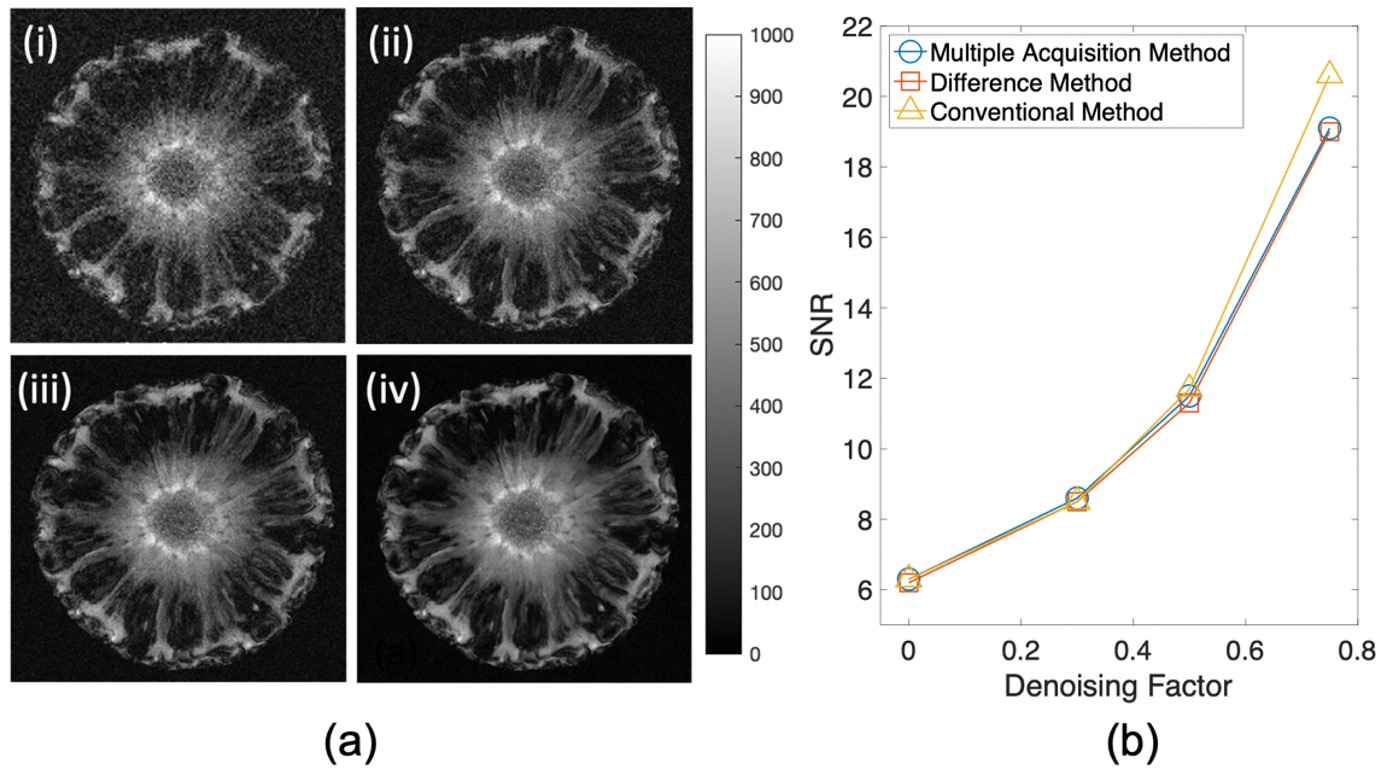
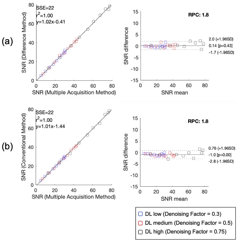
Figure 1 demonstrates subjective and quantitative increases in SNR in the pineapple images with increasing denoising factors using the DL reconstruction.Figure 2 shows excellent agreement in SNR measurements of sphere phantom images among three methods with different denoising levels.
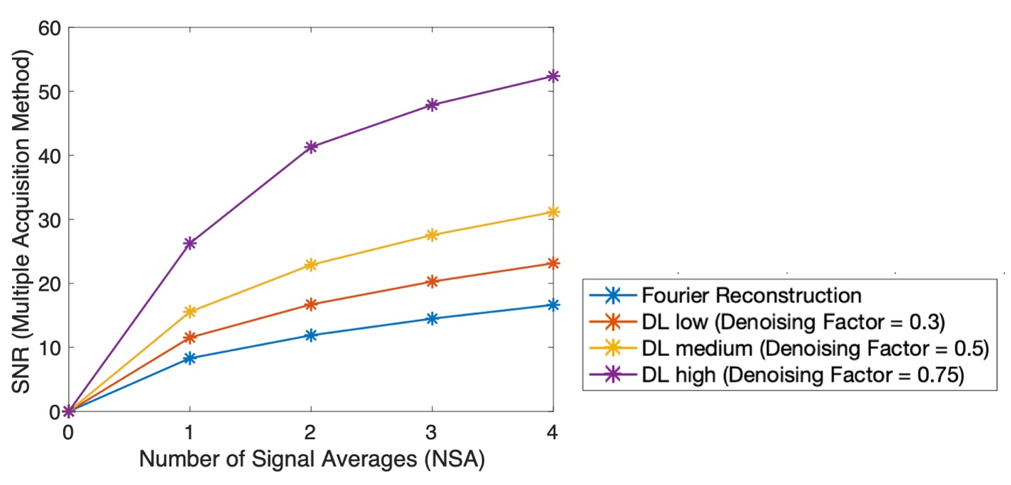
Figure 3 shows measured SNR in sphere phantom images as a function of NSA, demonstrating that the DL reconstruction enables similar SNR to Fourier reconstruction from faster acquisitions.
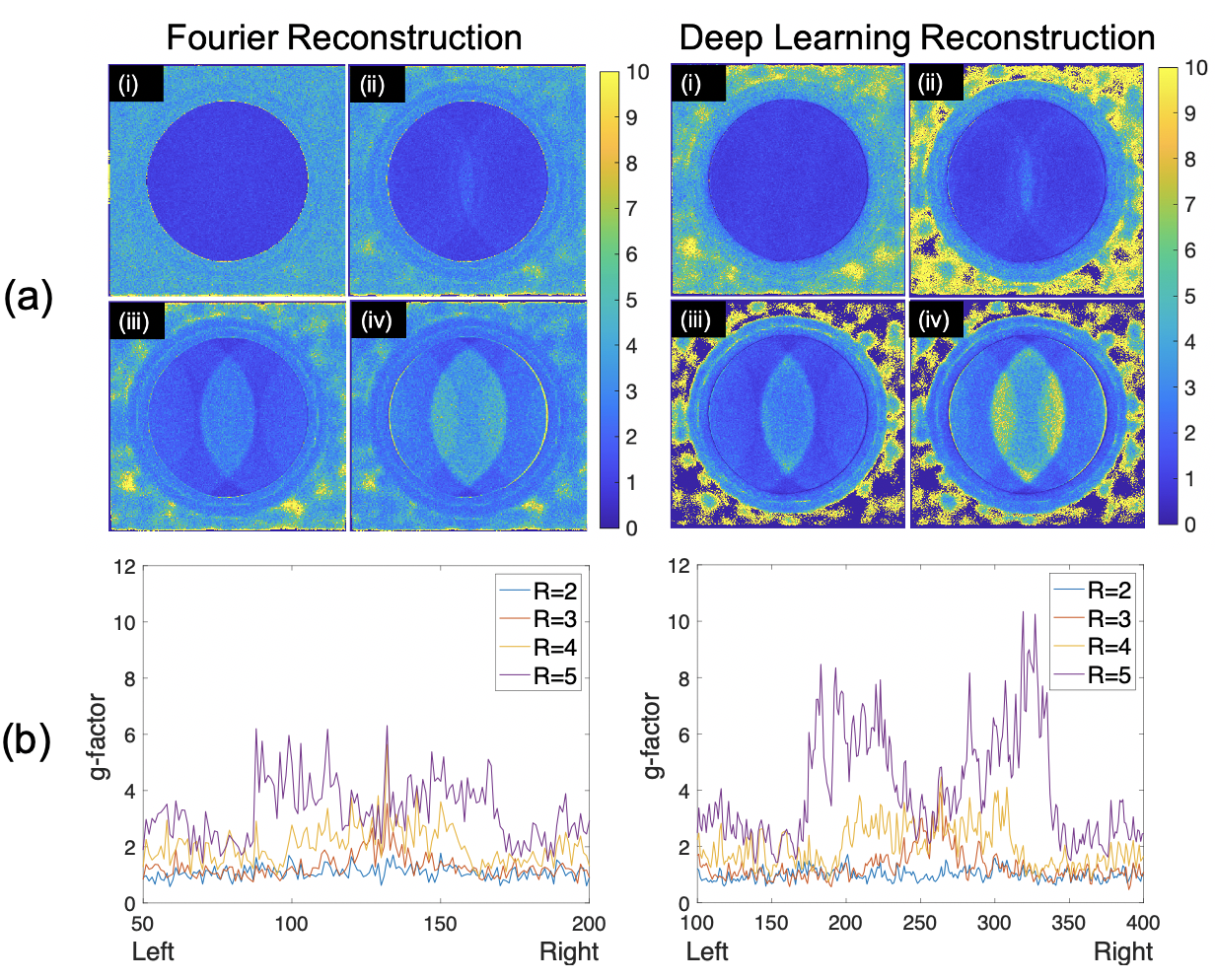
Figure 4 shows the g-factor maps of Fourier reconstructed images and DL reconstructed images, demonstrating that DL reconstructed images have a similar pattern of g-factor performance as Fourier reconstructed images, although worse g-factor performance at higher acceleration.
Discussion/Conclusions
In this work, we evaluated three practical approaches for the evaluation of SNR performance of DL reconstructed MR images. The multiple-acquisition method, difference method, and conventional method all have excellent agreement for both Fourier and DL reconstructions. This implies that both difference method and conventional method (in the absence of parallel imaging acceleration) may be applicable to DL reconstructed images. We also conclude that the difference method is a valid approach to measure SNR in both Fourier and DL reconstructed images accelerated using parallel imaging.We also demonstrated that images accelerated using parallel imaging show a similar g-factor pattern in DL and Fourier reconstructed images. Interestingly, we also found that at high acceleration factors, DL reconstructed images have worse g-factor performance. However, the g-factor performances of two reconstruction methods are similar at low-moderate acceleration factors.
Limitations of this study include consideration of a single DL-based reconstruction method, and imaging in only phantoms. Future work will include in-vivo imaging.
Acknowledgements
We wish to acknowledge support from GE Healthcare who provides research support to the University of Wisconsin. Dr. Reeder is a Romnes Faculty Fellow and has received an award provided by the University of Wisconsin-Madison Office of the Vice Chancellor for Research and Graduate Education with funding from the Wisconsin Alumni Research Foundation.
References
1. A. Pal and Y. Rathi, “A review of deep learning methods for MRI reconstruction,” arXiv:2109.08618v1 [eess.IV], Sep. 2021.
2. E. R. McVeigh, R. M. Henkelman, and M. J. Bronskill, “Noise and filtration in Magnetic Resonance Imaging,” Medical Physics, vol. 12, no. 5, pp. 586–591, 1985.
3. R. M. Henkelman, “Measurement of signal intensities in the presence of noise in Mr Images,” Medical Physics, vol. 12, no. 2, pp. 232–233, 1985.
4. O. Dietrich, J. G. Raya, S. B. Reeder, M. Ingrisch, M. F. Reiser, and S. O. Schoenberg, “Influence of multichannel combination, parallel imaging and other reconstruction techniques on MRI noise characteristics,” Magnetic Resonance Imaging, vol. 26, no. 6, pp. 754–762, 2008.
5. S. B. Reeder, B. J. Wintersperger, O. Dietrich, T. Lanz, A. Greiser, M. F. Reiser, G. M. Glazer, and S. O. Schoenberg, “Practical approaches to the evaluation of Signal-to-noise ratio performance with parallel imaging: Application with cardiac imaging and a 32-channel cardiac coil,” Magnetic Resonance in Medicine, vol. 54, no. 3, pp. 748–754, 2005.
6. K. P. Pruessmann, M. Weiger, M. B. Scheidegger, and P. Boesiger, “Sense: Sensitivity encoding for Fast Mri,” Magnetic Resonance in Medicine, vol. 42, no. 5, pp. 952–962, 1999.
7. R. M. Lebel. “Performance characterization of a novel deep learning-based MR image reconstruction pipeline,” arXiv:2008.06559 [eess.IV], Aug. 2020.
Figures