4044
Low-Rank Inversion Reconstruction for Through-Plane Accelerated Radial MR Fingerprinting at 0.35T
Nikolai J Mickevicius1 and Carri K Glide-Hurst1
1Department of Human Oncology, University of Wisconsin-Madison, Madison, WI, United States
1Department of Human Oncology, University of Wisconsin-Madison, Madison, WI, United States
Synopsis
To reduce scan time, methods to accelerate hybrid phase encoded/non-Cartesian MR fingerprinting (MRF) acquisitions for variable density spiral acquisitions have recently been developed. These methods are not applicable to MRF acquisitions wherein a single k-space spoke is acquired per frame. Therefore, we describe, implement, and test a low-rank inversion method on a 0.35T MR-guided radiation therapy system to resolve MR fingerprinting contrast dynamics from through-plane accelerated Cartesian/radial measurements.
Purpose
To reduce the scan time of MRF acquisitions with in-plane radial and through-phase encoded (i.e., stack-of-stars) k-space coverage for $$$T_1$$$ and $$$T_2$$$ mapping on a 0.35T MR-guided radiotherapy system.Introduction
Magnetic resonance fingerprinting (MRF)[1] is a novel technique to rapidly measure quantitative tissue parameters such as longitudinal and transverse relaxation rates $$$T_1$$$ and $$$T_2$$$, respectively. In an increasing number of implementations, MRF is performed with a single in-plane radial k-space spoke acquired per frame[2-6]. The contrast dynamics resulting from the continuously changing flip angle are then resolved with a constrained low-rank reconstruction. Extension of this acquisition scheme to through-plane accelerated 3D stack-of-stars MRF acquisitions is non-trivial owing to the aliasing that is present along the slice dimension. Here, a novel reconstruction approach to reconstructing high quality $$$T_1$$$ and $$$T_2$$$ maps from these highly accelerated acquisitions is described.Methods
The acquisition scheme can be visualized in Figure 1. A controlled aliasing in parallel imaging (CAIPIRINHA)[7] sampling of phase encoding partitions from frame-to-frame was performed similar to Ma et. al.[8] For an acceleration factor along the phase encoding direction of $$$R=2$$$, the relative phase between the aliased slices is modulated by $$$\pi$$$ from spoke to spoke. As demonstrated in Yutzy et. al.[9] this phase modulation, given by $$$\mathbf{\Theta}$$$, can be used to improve the conditioning of the reconstruction for through-plane accelerated acquisitions. The reconstruction problem to recover $$$\mathbf{\alpha} \in \mathbb{C}^{N^2R \times K}$$$, which is the low-dimensional representation of $$$R$$$ aliased $$$N \times N$$$ images, is shown below. Here, $$$K$$$ is the rank of the temporal subspace $$$\mathbf{\Phi} \in \mathbb{C}^{T \times K}$$$, where $$$T$$$ is the number of frames in the MRF acquisition and $$$K<<T$$$.$$\underset{\alpha}{\operatorname{argmin}} \left\lVert \mathbf{S}\mathbf{\Theta}\mathbf{F}\mathbf{\Phi}\mathbf{C}\mathbf{\alpha}-\mathbf{y} \right\rVert_2^2 + \lambda \sum_r \left\lVert \mathcal{R}_r (\alpha)\right\rVert_*$$
In the data consistency term, $$$\mathbf{F}$$$ represents the non-uniform fast Fourier transform operator, $$$\mathbf{C}$$$ contains the coil sensitivity maps for each aliased slice, $$$\mathbf{S}$$$ is an operator to sum over the aliased slice locations, and $$$\mathbf{y}$$$ is the measured k-space data. Similar to Tamir et. al.[10] the regularization term imposes a locally low rank (LLR) constraint to improve the condition of the inverse problem. This problem is solved using an alternating direction method of multipliers algorithm using Python and PyTorch for GPU acceleration. A multi-contrast non-local means (NLM) denoising algorithm[11] was applied to $$$\alpha$$$ following reconstruction.
Experiments were performed on an integrated 0.35T MRI and radiotherapy delivery system. As we have previously demonstrated that a linear reconstruction of fully phase encoded (i.e., $$$R=1$$$) MRF data agrees well with ground truth measurements[6], these will serve as the baseline reference for our novel reconstruction for $$$R>1$$$. $$$R=1$$$ and $$$R=2$$$ data were acquired in a standardized system phantom and in the brain and pelvis of consenting healthy volunteers. The mean and standard deviations of the $$$T_1$$$ and $$$T_2$$$ estimates between $$$R=1$$$ and $$$R=2$$$ were compared using paired t-tests.
Results
Numerical results from the phantom MRF experiments can be seen in Figure 2. Near perfect correlations between the fully sampled and accelerated MRF acquisitions were observed for both the $$$T_1$$$ (0.997) and $$$T_2$$$ (0.999) times. No significant differences between the $$$R=1$$$ and $$$R=2$$$ acquisitions was observed (P=0.41 for $$$T_1$$$ and P=0.36 for $$$T_2$$$). The mean absolute percent error in $$$T_1$$$ and $$$T_2$$$ were 5.6% and 2.9%, respectively, between $$$R=1$$$ and $$$R=2$$$ reconstructions. The standard deviations in $$$T_1$$$ and $$$T_2$$$ time estimates for $$$R=2$$$ reconstructions were significantly lower than those from the linear $$$R=1$$$ reconstructions (P=0.02 and P=0.03, respectively).In vivo results can be seen in Figures 3-5. In Figure 3, the $$$K=5$$$ subspace coefficient images can be seen for the linear $$$R=1$$$ reconstruction and the LLR+NLM $$$R=2$$$ reconstruction along with $$$T_1$$$ and $$$T_2$$$ maps. Sagittal and coronal reformats of the quantitative relaxation time maps can also be seen in Figure 4. These data demonstrate the capability of the $$$R=2$$$ reconstruction to yield high quality $$$T_1$$$ and $$$T_2$$$ maps visually comparable to those from the established linear $$$R=1$$$ reconstruction. Quantitative results can be seen in Figure 5, wherein the mean and standard deviations from several in vivo regions of interest are plotted. No significant differences were observed between $$$R=1$$$ and $$$R=2$$$ measurements with P=0.12 for $$$T_1$$$ and P=0.58 for $$$T_2$$$.
Discussion
This initial technical study on a novel algorithm for through-plane accelerated MRF demonstrated for the acquisition of volumetric $$$T_1$$$ and $$$T_2$$$ maps in only 3 minutes on a 0.35T MR-linac system. The benefits observed at low magnetic field strength with radial k-space coverage here may also extend to MRF acquisitions made with more-common variable density spiral trajectory and higher magnetic field strengths. The technologies proposed here will allow for the acquisition of longitudinal multi-parametric quantitative imaging throughout the course of radiation therapy treatment without burdening the patient with excessively long scan times.Acknowledgements
No acknowledgement found.References
- D. Ma et al., “Magnetic resonance fingerprinting,” Nature, vol. 495, no. 7440, pp. 187–192, Mar. 2013, doi: 10.1038/nature11971.
- J. Assländer, M. A. Cloos, F. Knoll, D. K. Sodickson, J. Hennig, and R. Lattanzi, “Low rank alternating direction method of multipliers reconstruction for MR fingerprinting,” Magn. Reson. Med., Mar. 2017, doi: 10.1002/mrm.26639.
- G. L. da Cruz, A. Bustin, O. Jaubert, T. Schneider, R. M. Botnar, and C. Prieto, “Sparsity and locally low rank regularization for MR fingerprinting,” Magn. Reson. Med., vol. 81, no. 6, pp. 3530–3543, Jun. 2019, doi: 10.1002/MRM.27665.
- G. Cruz, O. Jaubert, T. Schneider, R. M. Botnar, and C. Prieto, “Rigid motion-corrected magnetic resonance fingerprinting,” Magn. Reson. Med., vol. 81, no. 2, pp. 947–961, Feb. 2019, doi: 10.1002/MRM.27448.
- T. Bruijnen et al., “Technical feasibility of magnetic resonance fingerprinting on a 1.5T MRI-linac,” Phys. Med. Biol., vol. 65, no. 22, pp. 22–23, Nov. 2020, doi: 10.1088/1361-6560/abbb9d.
- N. J. Mickevicius, J. P. Kim, J. Zhao, Z. S. Morris, N. J. Hurst, and C. K. Glide-Hurst, “Toward magnetic resonance fingerprinting for low-field MR-guided radiation therapy,” Med. Phys., Sep. 2021, doi: 10.1002/MP.15202.
- F. A. Breuer, M. Blaimer, R. M. Heidemann, M. F. Mueller, M. A. Griswold, and P. M. Jakob, “Controlled aliasing in parallel imaging results in higher acceleration (CAIPIRINHA) for multi-slice imaging.,” Magn. Reson. Med., vol. 53, no. 3, pp. 684–691, Mar. 2005, doi: 10.1002/mrm.20401.
- D. Ma et al., “Fast 3D magnetic resonance fingerprinting for a whole‐brain coverage,” Magn. Reson. Med., vol. 79, no. 4, pp. 2190–2197, Apr. 2018, doi: 10.1002/mrm.26886.
- S. R. Yutzy, N. Seiberlich, J. L. Duerk, and M. A. Griswold, “Improvements in multislice parallel imaging using radial CAIPIRINHA.,” Magn. Reson. Med., vol. 65, no. 6, pp. 1630–1637, Jun. 2011, doi: 10.1002/mrm.22752.
- J. I. Tamir et al., “T 2 shuffling: Sharp, multicontrast, volumetric fast spin‐echo imaging,” Magn. Reson. Med., vol. 77, no. 1, pp. 180–195, Jan. 2017, doi: 10.1002/mrm.26102.
- J. V. Manjón, J. Carbonell-Caballero, J. J. Lull, G. García-Martí, L. Martí-Bonmatí, and M. Robles, “MRI denoising using Non-Local Means,” Med. Image Anal., vol. 12, no. 4, pp. 514–523, Aug. 2008, doi: 10.1016/J.MEDIA.2008.02.004.
Figures
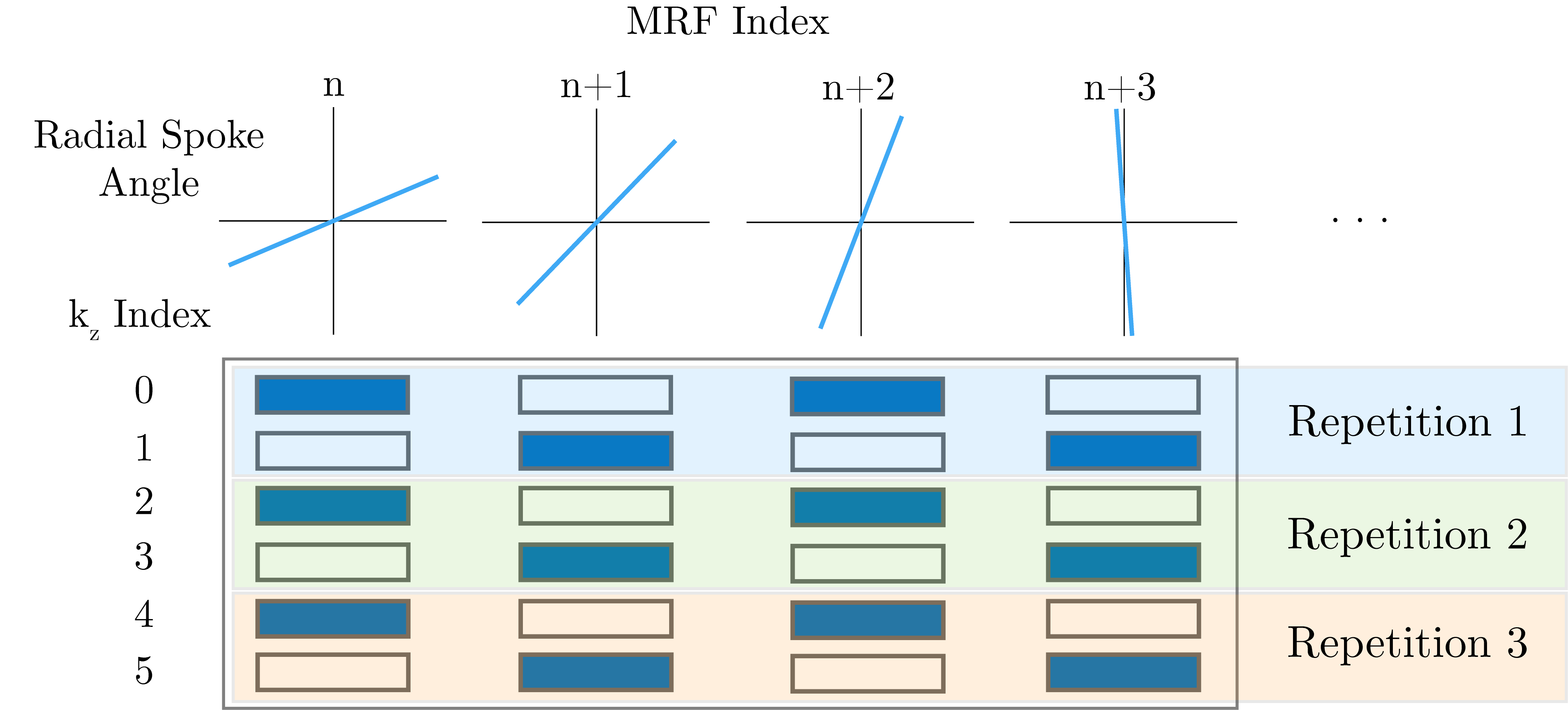
Figure 1. Controlled aliasing in parallel imaging (CAIPI or CAIPIRINHA) sampling for stack-of-stars MR fingerprinting. At each MRF Index, n, along the variable flip angle pattern, a unique spoke angle is acquired by incrementing the angle by a tiny golden angle increment. For 2x through-plane accelerated acquisition as shown here, the phase encoding index ($$$k_z$$$) alternates between the nearest even and odd sampling index for a given repetition. Within each MRF index, uniform k-space sampling along $$$k_z$$$ is achieved.
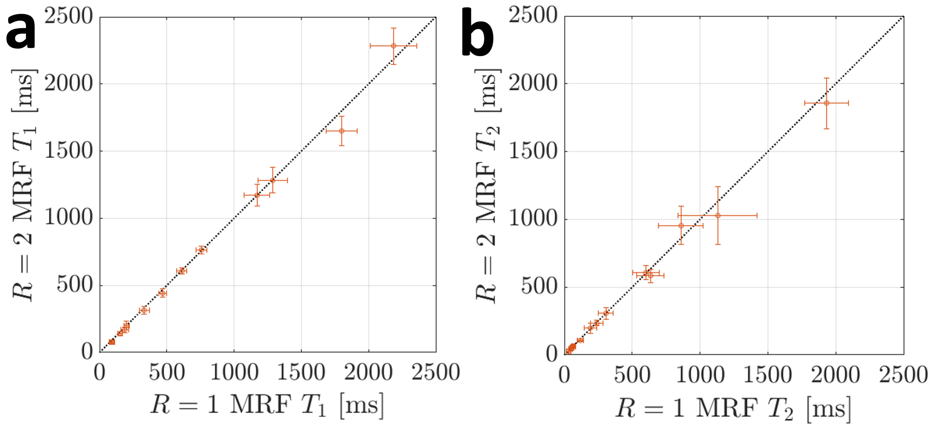
Figure 2. Differences in $$$T_1$$$ and $$$T_2$$$ between the fully partition encoded ($$$R=1$$$) stack-of-stars MRF and the two-times accelerated ($$$R=2$$$) datasets. The mean values are shown along with standard deviation within each sphere of the NIST/ISMRM system phantom. The identity line is plotted for reference.

Figure 3. Brain and pelvis in vivo results for fully sampled ($$$R=1$$$) linear reconstruction and accelerated ($$$R=2$$$) locally low rank (LLR) regularized reconstructions with non-local means (NLM) denoising. The singular value (SV) images are shown for each dataset. Note that each image is windowed individually. $$$T_1$$$ and $$$T_2$$$ maps fit via matching of the SV images and the dictionary are shown on the right.

Figure 4. Axial, sagittal, and coronal views of the 3D $$$T_1$$$ and $$$T_2$$$ maps from the $$$R=1$$$ and $$$R=2$$$ MRF acquisitions. Comparable image quality of the $$$T_1$$$ and $$$T_2$$$ maps can be seen between $$$R=1$$$ and $$$R=2$$$ reconstructions.

Figure 5. In vivo $$$T_1$$$ and $$$T_2$$$ time comparison between fully sampled ($$$R=1$$$) and accelerated ($$$R=2$$$) datasets within regions of interest (ROIs) in white matter (WM), gray matter (GM), musculoskeletal (MSK) tissue, the central zone (CZ) of the prostate, and in the hip bone marrow. The top row (a,b) shows the $$$T_1$$$ and $$$T_2$$$ values from every voxel within all regions of interest. The bottom row (c,d) shows the mean $$$T_1$$$ and $$$T_2$$$ values along with their standard deviations within each of these ROIs.
DOI: https://doi.org/10.58530/2022/4044