4003
Deep learning identification of clear cell renal carcinoma cancer using MR imaging1Radiology, UT southwestern medical center, Dallas, TX, United States
Synopsis
Clear cell renal carcinoma cancer (ccRCC) is the most common subtype among renal masses. ccRCC identification helps in decision making between active surveillance and definitive intervention. A clear cell likelihood score (ccLS) using subjective interpretation of multiparametric MRI by radiologists was proposed recently. In this study, we investigate whether deep learning (DL) using the three main MR sequences for ccLS can facilitate the diagnosis of ccRCC. We compared the results of twelve trained DL models with the reported ccLS performance. Our results demonstrate that DL may achieve a performance comparable to radiologists and provide useful information for identification of ccRCC.
Introduction
Renal cell carcinoma (RCC) is the most common type of kidney cancer (about 90%). Clear cell renal cell carcinoma (ccRCC) is the most common and aggressive histologic subtype of RCC (about 70%) 1, 2. Small-renal-masses (SRM, ≤4cm) account for over 50% of renal masses and encompass a broad disease spectrum from benign tumors (20%) to aggressive malignancies 1, 3. Active surveillance (AS) is an accepted management strategy for patients with SRMs and larger localized tumors (4 cm<T1b< 7cm), particularly those with comorbidities and limited life expectancy 4. Identification of ccRCC can help for deciding treatment between AS and definitive intervention 5. A qualitative 5-tier classification system, the clear cell likelihood score (ccLS), derived from multiparametric MRI using T2-weighted (T2w), T1-weighted (T1w) in-phase/opposed-phase (IP/OP), diffusion-weighted, and multi-phasic-contrast-enhanced MRI with a T1w fat-saturated spoiled-gradient-echo-sequence (FS-SPGR) was proposed to identify ccRCC 5. In this study, we investigated whether deep learning could facilitate the identification of ccRCC using the three most important sequences in the ccLS algorithm: T2w, T1w IP/OP, and contrast-enhanced T1w corticomedullary-phase (CMph) images.Methods
This retrospective study included subjects who under-went surgical resection of a renal mass and who had presurgical MR images available for analysis. Coronal T2w single-shot-fast-spin-echo images, axial T1w-IPOP images, and coronal (or axial) CMph images were acquired on different scanners (GE, Philips, and Siemens). The number of subjects for different sequences are summarized in Table 1. Subjects with a single tumor and tumor size less than 7 cm (T1a and T1b) were included in this study. The number of patients varied for different contrast due to missing series and motion artifacts. Tumor masks were manually drawn by an imaging specialist.A deep learning model, 2D Efficientnet (b0), was used to predict the probability of ccRCC using three different MR sequences: T2w, T1w-IPOP, and T1w-CM in Pytorch. For each contrast, three models were trained using different inputs: 1. the cropped image only (10 cm, 200x200 matrix); 2. the cropped image and the tumor mask; 3. the cropped image and a Gaussian weight (Gweight) as shown in Fig. 1a. The 2D-normalized-Gaussian-weight images with a size of 200 and a sigma of 4 were generated. The peak was located at the image center. In addition, a customized model, FusionNet, was trained using all images from three sequences in Fig. 1b. Four-fold-cross-validation was used to estimate the performance of each model. Tumor slices were selected for training. The images were divided into training, validation, and testing sets. The testing sets (20%) were separated based on subjects instead of slices to prevent the data leaking between training and testing stages. The remaining data were further divided into training (80%) and validation (20%) sets. The detailed information of different datasets is summarized in Table 1. The preprocessing steps included N4bias field correction, and z-score normalization. The data augmentation steps were randomly implemented in every epoch including 2D rotation (-10°~10°) and left-right flip. Batch size was 100 and the total number of epochs was 200.
ROC analysis was performed to calculate the area-under-curve (AUC) for each model. In addition, the metrics including accuracy, precision, sensitivity, and specificity were computed for each model. Slice-based metrics were first estimated based on the prediction of ccRCC for each slice. Furthermore, subject-based metrics were assessed based on the slice results using a threshold. The averaged probability of all tumor slices of each subject were computed and the testing subjects were identified as ccRCC when their probability was larger than a threshold, a mean of probability of all the testing subjects. For fusion, the averaged probability was computed from the top 20 probabilities of all combinations, and the threshold of 0.9 were used. DL Results were compared with reported performance of the ccLS criteria.
Results
Figure 2. shows the summary of mean AUCs for all cases. The T2w-Gweight model achieved the best subject-based results with 77% mean accuracy, 82% mean sensitivity, 72% mean specificity, and mean AUC of 0.77. These DL results are comparable to previously reported human results using ccLS 4/5 (79% mean accuracy, 78% mean sensitivity, 80% mean specificity) and ccLS 3/4/5 (77% mean accuracy, 95% mean sensitivity, 58% mean specificity)6. The mean metrics for T2w and fusion are summarized in Table 2. Of the three MR sequences, T2w and T1w-CMph images achieved a better prediction of ccRCC than T1w-IPOP images 7. The fusion model improved the slice-based performance of prediction and achieve a T2w-comparable subject-based performance in Fig.2.Discussion/Conclusion
Our results demonstrate that deep learning techniques have a potential to facilitate the prediction of ccRCC histology with MRI. The fusion model, combining the different contrasts on a subject level, achieved the prediction performance comparable to that using T2w images only. We will further investigate the feasibility to combine all the contrasts together in different ways in future. The deep learning model using Gaussian weight still required some human input for locating the center of tumors, which may be more feasible than drawing the whole 3D tumor masks. Optimization of deep learning models will require further validation in a larger cohort of subjects.Acknowledgements
This project is supported by NIH grants R01CA154475, U01CA207091, and P50CA196516. We thank Ayobami Odu for image annotation.
References
1. Weikert, S. and B. Ljungberg, Contemporary epidemiology of renal cell carcinoma: perspectives of primary prevention. World J Urol, 2010. 28(3): p. 247-52.
2. Campbell, S., et al., Renal Mass and Localized Renal Cancer: AUA Guideline. J Urol, 2017. 198(3): p. 520-529.
3. Frank, I., et al., Solid renal tumors: an analysis of pathological features related to tumor size. J Urol, 2003. 170(6 Pt 1): p. 2217-20.
4. Sebastia, C., et al., Active surveillance of small renal masses. Insights Imaging, 2020. 11(1): p. 63.
5. Johnson, B.A., et al., Diagnostic performance of prospectively assigned clear cell Likelihood scores (ccLS) in small renal masses at multiparametric magnetic resonance imaging. Urol Oncol, 2019. 37(12): p. 941-946.
6. Canvasser, N.E., et al., Diagnostic Accuracy of Multiparametric Magnetic Resonance Imaging to Identify Clear Cell Renal Cell Carcinoma in cT1a Renal Masses. J Urol, 2017. 198(4): p. 780-786.
7. Steinberg, R.L., et al., Prospective performance of clear cell likelihood scores (ccLS) in renal masses evaluated with multiparametric magnetic resonance imaging. Eur Radiol, 2021. 31(1): p. 314-324.
Figures
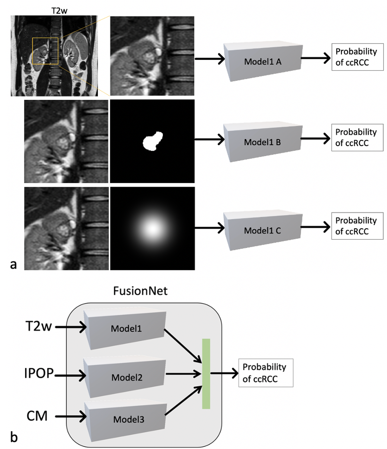
Figure 1. Diagrams of deep learning (DL) models for different datasets. a. three DL models for T2w datasets with different inputs: cropped image only for model1A, cropped image and mask for model1B, and cropped image with Gaussian weighting for model1C; b. a FusionNet model by combining three contrast images together. T2w, T2-weighted image; IPOP, T1-weighted inphase and outphase images; CM, DCE-MRI corticomedullary phase image.
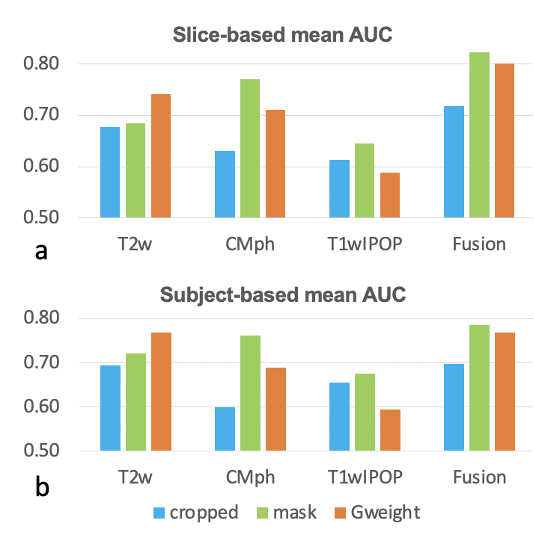
Figure 2. Summary of prediction results using different images and CNN models. a. Summary of slice-based mean AUCs using T2w, T1w CM phase, T1wIPOP images, and all three sequences combined (Fusion); b. Corresponding subject-based mean AUCs. Cropped represents the results from model1A in Fig. 1; Mask represents the results from model1B in Fig. 1; Gweight represents the results from model1C in Fig. 1. AUC, area under curve.

Table 1. Summary of data information for four DL models with four-fold cross validation.
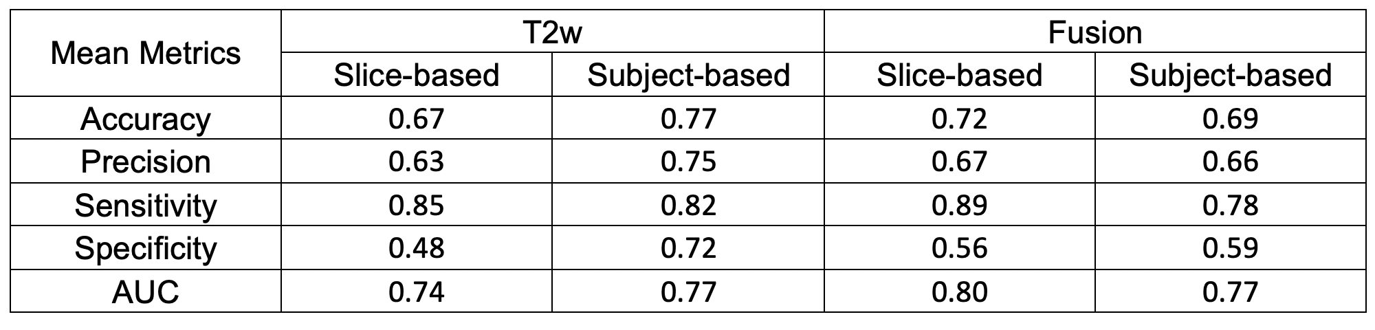
Table 2. Summary of the mean metrics of predictions for T2w and Fusion using a Gaussian weight.