Introduction and Motivation

Multiple Sclerosis (MS) is a neurodegenerative disease marked by inflammation, demyelination, neuronal loss and axonal degeneration. The pathological features of MS manifest in white matter (WM) and gray matter (GM) as both focal plaques and diffuse tissue injury, varying with MS phenotype, disease duration and type of disease modifying therapy¹.

Apparent transverse relaxation time (T₂^*) and longitudinal relaxation time (T₁) are quantitative relaxometry metrics sensitive to myelin and iron in the brain. T₂^* and T₁ can be applied to assess the extent and spatial distribution of diffuse WM pathology in MS². Histopathological and imaging studies of post-mortem MS brain tissue have revealed two distinct types of diffuse non-plaque WM changes: normal-appearing WM (NAWM) and dirty-appearing WM (DAWM). NAWM is characterized by demyelination, inflammation, axonal loss, and lengthened T₂^* and T₁ times^{3, 4}. In contrast, DAWM shows greater demyelination, greater increase in T₂^* and T₁ times, and typically comprises regions with indefinite boundaries³. However, the optimal quantitative MRI method for unique discrimination of DAWM from NAWM and an understanding of the underlying MS pathological substrates is an ongoing area of investigation.

The motivation for this work was to apply high-resolution, robust 7T quantitative T₂^* and T₁ mapping of post-mortem MS brain tissue to identify and discriminate NAWM and DAWM.

Methods

Brain Samples: Nine post-mortem, human cerebral brain sections were obtained from the Douglas-Bell Canada Brain Bank (duration of formalin fixation ≥ 10 years). Specifically, 6 sections were obtained from two MS patient donors (Patient #1: Frontal, middle and caudal large sections; Patient #2: Frontal small, frontal large and caudal sections) and 3 sections were obtained from two healthy control donors (Control #1: Frontal and caudal sections; Control #2: Caudal section).

MR Scanning: Brain sections were scanned using a Siemens 7T Scanner (MAGNETOM Terra) with a 1Tx/32Rx head coil (Nova Medical). Acquisitions included a slab-selective 3D Multi-Echo (ME) GRE sequence (0.32mm³, TR = 46ms, TE = [6.84, 11.57, 16.30, 21.03, 25.76, 30.49]ms, FA = 15^o, 25 averages) and a 3D MP2RAGE sequence (0.32x0.32x0.64mm³, TR/TE = 3000/2.08ms, Turbo Factor = 24, echo spacing = 6.6ms, FA1/FA2 = 8/8^o, TI1/TI2 = 183/900ms, 25 averages). A 2.5mm³ B₁⁺ map was acquired using Siemens’ Turbo-Flash B₁⁺ mapping protocol.

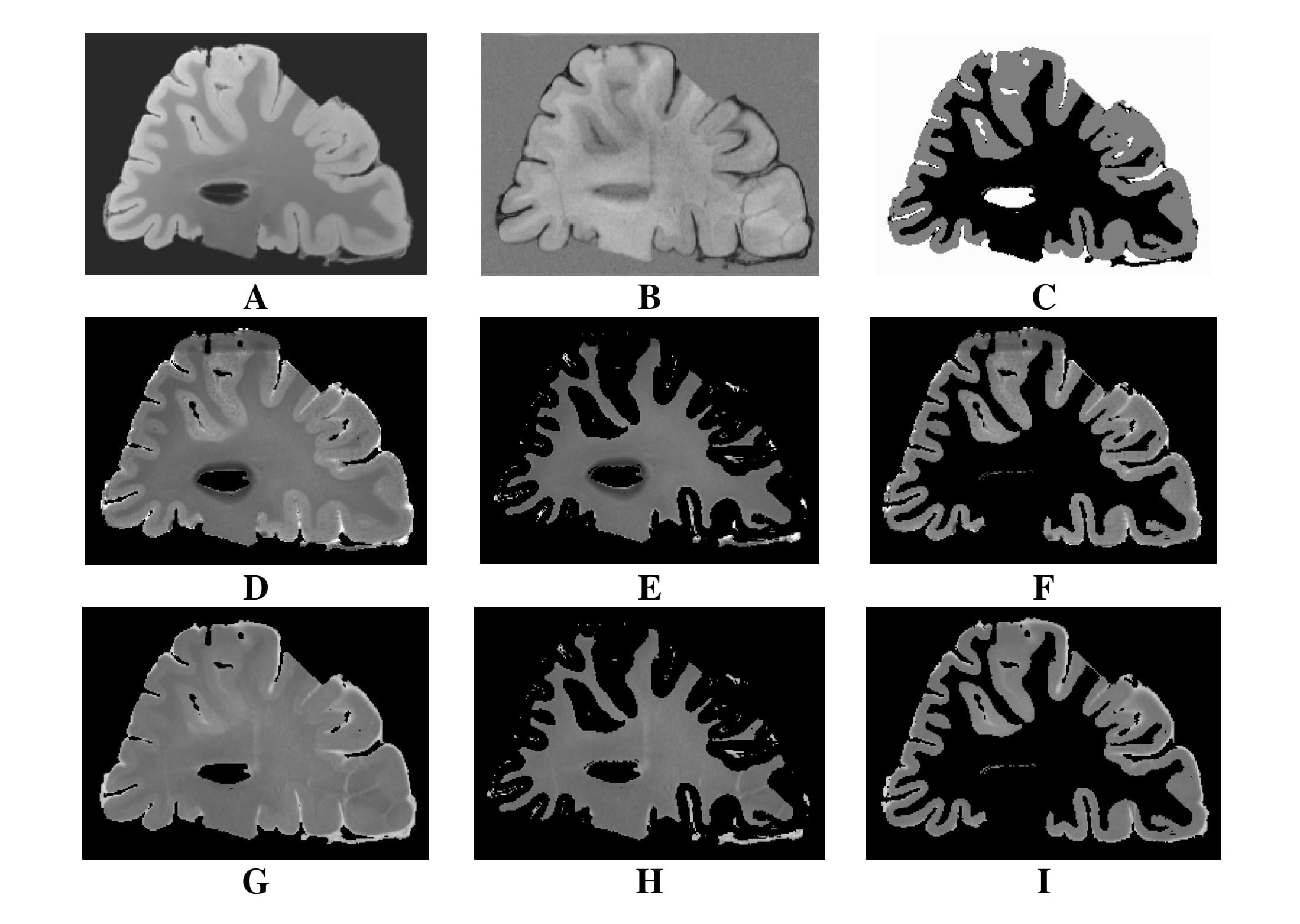
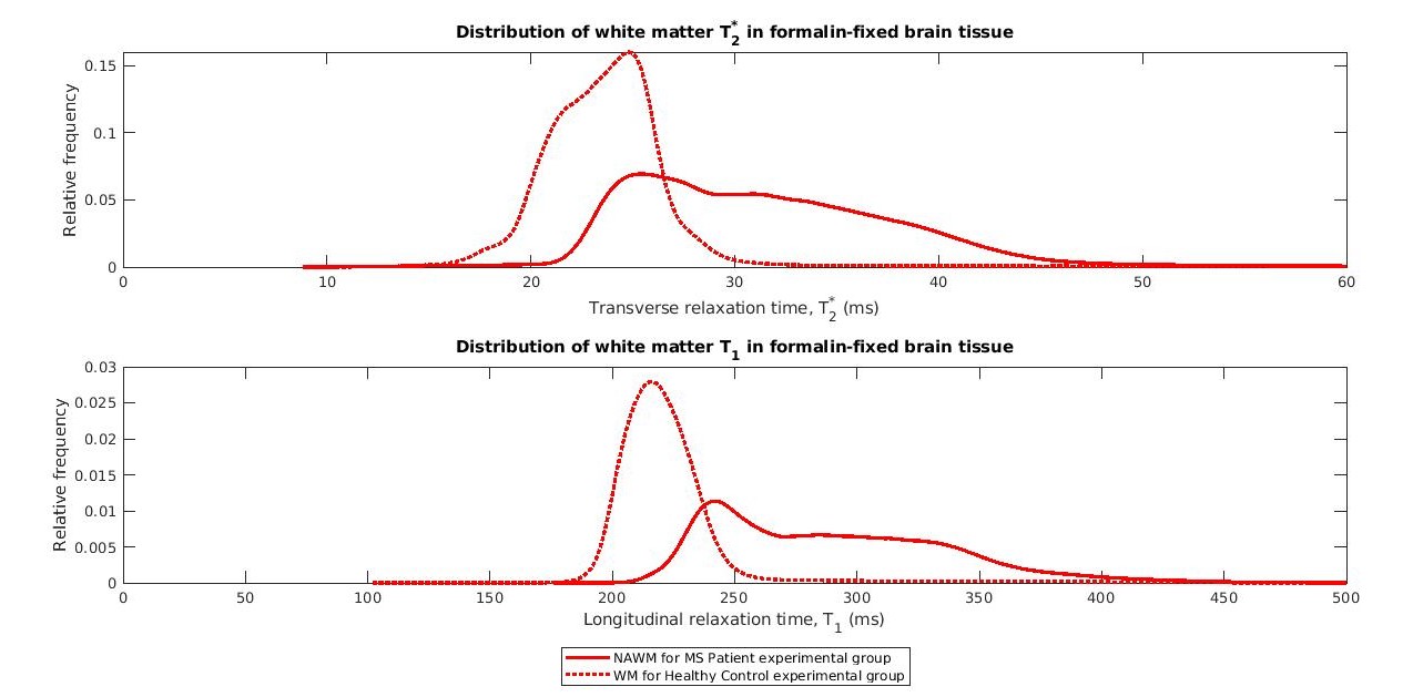
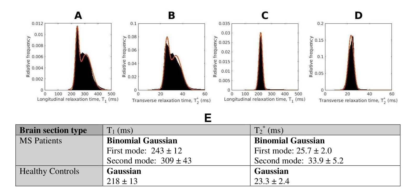
Data Processing: For each 3D-MP2RAGE measurement, a T₁ map was computed using Siemens’ MP2RAGE-based T₁ fitting algorithm. Individual T₁ maps and ME-GRE magnitude images were averaged to yield high SNR T­₁ maps and ME-GRE images for each brain section. The averaged T₁ data was upsampled and registered to the ME-GRE data using FLIRT (FSL, v7.2). Based on averaged ME-GRE magnitude data, T₂^* maps were computed using a voxel-wise non-linear, least-squares fitting approach in MATLAB (R2020b, Mathworks). To extract tissue-specific T₁ and T₂^* maps, the first echo image of the averaged ME-GRE was used to segment GM and WM, via the ilastik Pixel Classification workflow⁵ (Figure 1). Next, normalized, smoothed T₁ and T₂^* distributions in WM were generated from the MS patient and healthy control experimental groups (Figure 2). The distributions were fitted with bimodal and unimodal Gaussian functions to extract unique peak positions (Figure 3). Given the bimodal T₂^* and T₁ distributions for the MS patient group, the first (lower) and second (higher) modes were assumed to arise from the presence of NAWM and DAWM respectively. This assumption was made since DAWM is expected to entail a greater increase in T₂^* and T₁ compared to NAWM. To that end, “NAWM” here refers to all non-plaque WM outside the region classified as DAWM.

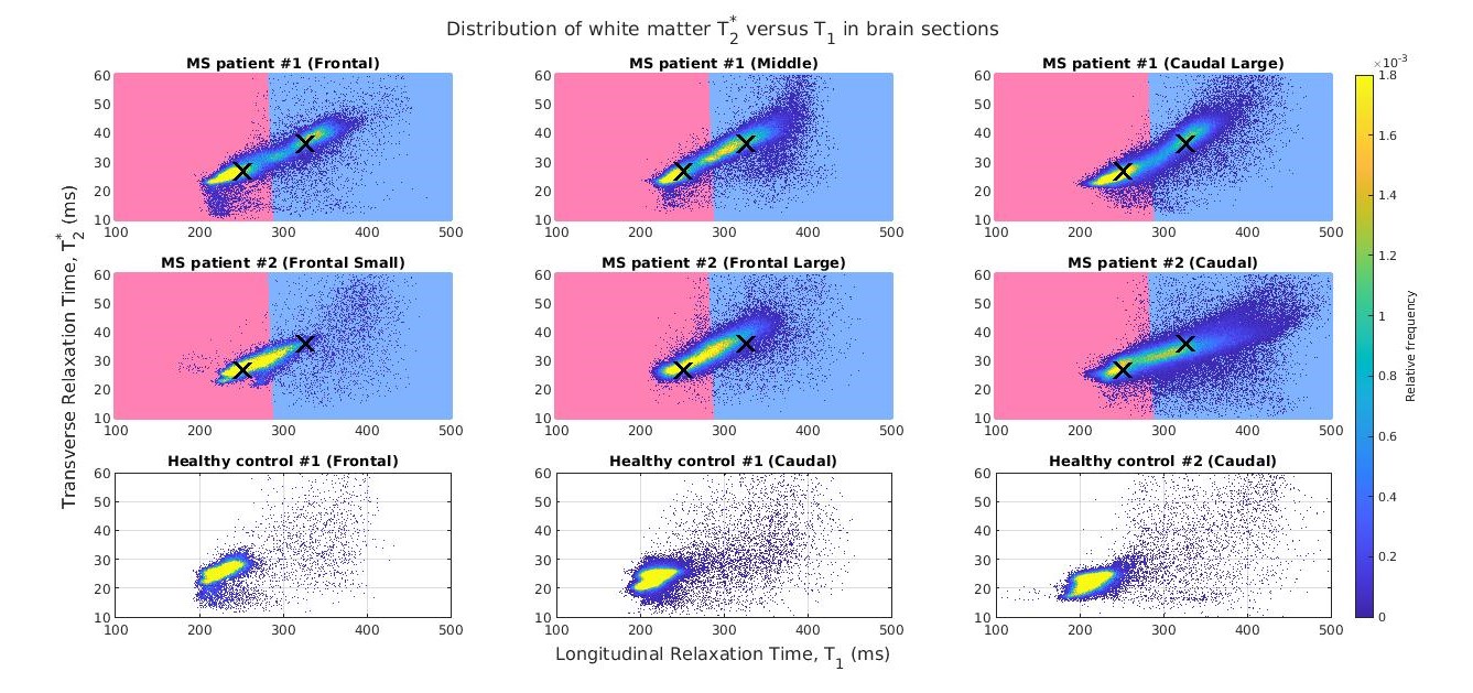
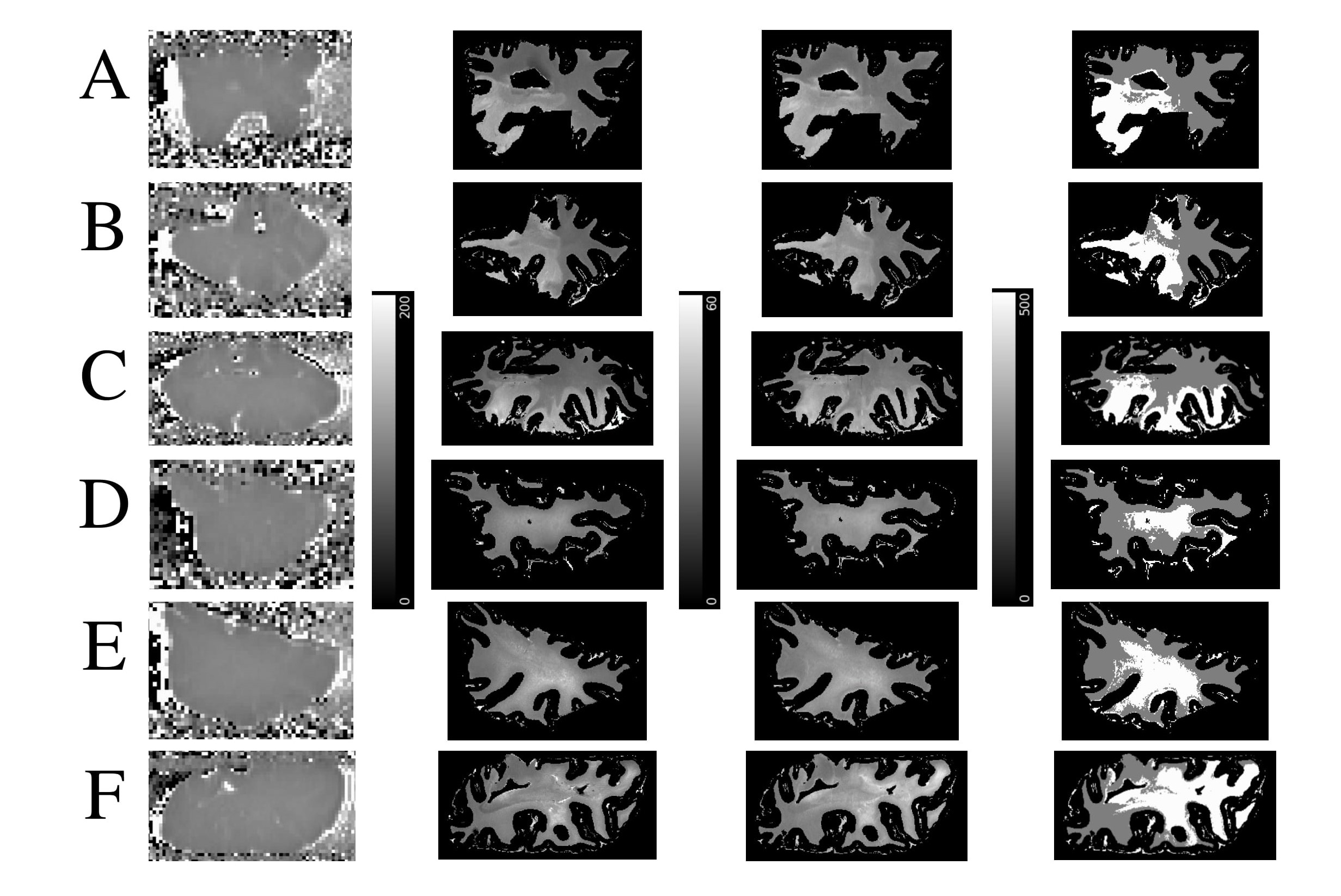
Classification: K-means clustering (k = 2) was applied to the MS tissue T₁ and T₂^* 2D data to create a classifier capable of discriminating between apparent NAWM and DAWM. For each brain section, a bivariate histogram of T₂^* versus T₁ was plotted (Figure 4) and clusters of T₂^*-T₁ values representative of DAWM (blue) and NAWM (pink) were indicated. A mask showing the spatial distribution of DAWM was also generated (Figure 5).

Results and Discussion

T₂^* and T₁ distributions in the MS patient group were lower in peak height, broader and shifted to longer relaxation time values compared to those of the healthy control group (Figure 3E). The broader distributions suggest heterogeneity of non-plaque abnormal WM⁶. The difference in NAWM and DAWM T₁ and T₂^* peak positions reflects the impact of myelin phospholipid damage³ on DAWM.

Bivariate T₂^*-T₁ relative frequency histograms (Figure 4) revealed two distinct hyperintensities in MS tissue which were not present in control tissue. The hyperintensities were demarcated by a linear decision boundary (approximately T₁ = 289 ms) calculated with K-means clustering. Mean (T₁, T₂^*) positions for the k-means clusters representative of NAWM and DAWM were (250, 26.7)ms and (325, 36.1)ms respectively.

The DAWM regions detected by the K-means classifier were located in periventricular WM (Figure 5), consistent with results of MS histopathological studies³. In most MS sections (A, B, F), DAWM did not have ill-defined borders but, rather, was well-delineated, comprising nearly half the tissue slab area. These findings support the joint use of 7 T T₂^* and T₁-based relaxometry approaches for identifying NAWM and DAWM pathology in MS. More definitive support based on ex-vivo histological myelin staining is underway, as a topic of our future work.

Acknowledgements

We gratefully acknowledge the Douglas-Bell Canada Brain Bank as the source of formalin fixed cerebral human brain tissue used in our work.