3946
Iterative MR-Electrical Properties Tomography using physics-based deep learning1DIIES, Università Mediterranea di Reggio Calabria, Reggio di Calabria, Italy, 2Computational Imaging Group for MR Diagnostics & Therapy, Center for Image Sciences, Utrecht University, Utrecht, Netherlands
Synopsis
We introduce for the first time an iterative MR electrical properties tomography reconstruction method by exploiting a cascade of multi-layer convolutional neural networks (CNNs) able to learn spatial priors in an iterative fashion, alternated with physics-based gradient descent direction calculations. This method was tested on 2D simulated human brain data. The presented results demonstrate the feasibility of this methodology to reconstruct conductivity and permittivity maps at 128MHz. Ultimately, this method allows computational advantages compared to standard contrast source inversion electrical properties tomography (CSI-EPT), i.e. faster reconstructions, which will be extremely relevant when moving to 3D reconstructions.
INTRODUCTION
MR-Electrical Properties Tomography (MR-EPT) aims at non-invasive MR-based measurements of tissue electrical properties (EPs: conductivity, σ, and relative permittivity, εr)[1]. To avoid the main issue of noise amplification of Helmholtz’s based methods, iterative-based reconstruction methods have been proposed, where the minimization of the cost function is achieved by gradient descent strategies[2]. However, these latter are significantly computationally demanding and may suffer from convergence issues due to local minima. Recently, deep-learning (DL) iterative image reconstruction methods have shown great potential in accelerating the reconstruction process while keeping knowledge of the forward model[3,4]. Inspired by these works, we present a physics-based iterative DL method for MR-EPT reconstructions, where the forward model is maintained, contrary to single-step direct DL approaches[5], and the contrast is updated by exploiting Convolutional-Neural-Networks (CNN).METHOD
Dataset and SimulationsStarting from a human brain model[7], 120 brain models were created by changing the white matter (WM), gray matter (GM), and cerebrospinal fluid (CSF) EPs values (ranging [5-20%] with respect to[8]) and by performing geometrical transformations, e.g. rotation of the brain model within the simulated coil. In total, 3240 2D maps were obtained ((Ntrain=2700, Ntest=540). Additionally, the proposed approach was tested on additional 20 brain models (Ntest=540 slices) with tumor-like anomalies (range: σ≈[0.7-1.2]S/m; εr≈ [54-80]) to test its robustness to unforeseen cases not included in training.
For EM simulations, a 2D configuration was considered without RF shield. A birdcage coil with 16 antenna arrays was used (radius r=0.37m[6]; each antenna was modelled as line sources). The magnetic field data were simulated using a full-wave forward simulator based on the method of moments[9] without superimposing noise.
Reconstruction
In standard iterative methods, the contrast update at the (k+1)th iteration is performed according to χk+1=χk+λkdk wherein χk is the contrast (χ=f(εr,σ)), λk is the step length, and dk is the descent gradient-determined direction at iteration kth. Instead, the proposed method starts from the computation of dk but updates the contrast profile χk by using a CNN[10]. The network architecture is the same among different iterations, while the network parameters are updated. At each iteration, the CNN learns an update of the contrast χk+1 by minimizing a loss function (half-mean-squared-error) between the predicted updated contrast χk+1 and the ground-truth (χtrue). The inputs of the network are the complex contrast profile at the iteration kth, χk, and the complex descend gradient-determined direction dk which enforces the physical model (Fig.1). Both in training and testing, a homogenous contrast map (χ0, σ≈0.56 S/m and εr≈45) was used as the initial guess.
RESULT AND DISCUSSION
Three iterations were considered as no further improvement was observed in the reconstructed conductivity/permittivity maps. The training time was about 3 hours. The reconstruction time for 1 model (27 slices), was about 8s (2.7s per iteration) on a workstation equipped with two Intel(R) Xeon(R) CPU E5-2687W v3(3.10 GHz) processors. This is much faster compared to standard CSI-EPT, which needed 4 minutes to reach the same reconstruction accuracy (27 slices, 16 iterations). The observed computational advantage will be especially relevant when moving to 3D, where 3D-CSI-EPT takes hours while the proposed method is expected to take few minutes only[11].In Fig.2, we show the reconstruction improvement on one slice for each iteration. For permittivity, the mean absolute percentage error (MAPE) improves from 8% to 4%; for conductivity it improves from 94% to 6%. These results also show good reconstruction quality at tissues boundaries. The higher error at the center of the brain (due to low electric field) is expected to be reduced when moving to 3D reconstructions[12].
In Fig. 3, permittivity/conductivity reconstructions for two different brain models are shown, demonstrating good reconstruction quality. As shown in the boxplots, the median MAPE across the 540 test-models is overall <10% for permittivity and <14% for conductivity in the WM, GM, CSF.
In Fig.4, permittivity/conductivity reconstructions for a brain tumor model show the capability of the presented approach to reconstruct EPs of structures not present in training. However, the reconstruction accuracy of the tumor is lower compared to other tissues: MAPE permittivity tumor 39%, MAPE conductivity tumor 37% (3rd iteration).
Finally, in Fig.5, permittivity/conductivity reconstructions for different tumor models are shown, together with the median MAPE across the whole testing dataset (median MAPE tumor permittivity≈40%, conductivity≈25%).
Ultimately, we can expect the reconstruction quality of the lesions to improve when anomalies are included in training. Alternatively, CSI-EPT can be run using the proposed results as initial guess[6]. As shown in Fig.4, this improves considerably the reconstruction accuracy of the tumor (MAPE permittivity 13%, MAPE conductivity 9%). By using the proposed method to provide an optimal initial guess for CSI-EPT, less iterations are needed, thus considerably reducing the CSI-EPT reconstruction time (otherwise hours for a head model)[11].
CONCLUSION
The proposed iterative MR-EPT with physics-based DL method is feasible and allows good quality permittivity/conductivity reconstructions for noiseless cases in few seconds. The key advantage is reducing the number of iterations and thus the reconstruction time compared to standard CSI-EPT. This is extremely relevant for 3D CSI-EPT reconstructions. Future work will extend to noisy data, 3D reconstructions and a more realistic coil setup.Acknowledgements
This work was supported by the European Commission, Fondo Sociale Europeo and Regione Calabria, POR-Calabria FSE 2014/2020. S.M. received funding from NWO, VENI grant n18078.References
[1] R. Leijsen, W. Brink, CAT van den Berg, A. Webb, R. Remis, Electrical properties tomography: “A methodological review”. Diagnostics, vol. 11, no. 2, 176, 2021.
[2] M. T. Bevacqua, G. G. Bellizzi, L. Crocco, L., T. Isernia, “A method for quantitative imaging of electrical properties of human tissues from only amplitude electromagnetic data”, Inverse Problems, vol. 35, 025006, 2019.
[3] J . Schlemper, J. Caballero, et al. A Deep Cascade of Convolutional Neural Networks for Dynamic MR Image Reconstruction. IEEE Trans Med Imag, 2018: 491-503.
[4] K. Hammernik, T. Klatzer et al. Learning a variational network for reconstruction of accelerated MRI data. Magn Res Med, 2018: 3055-3071.
[5] S. Mandija, E.F. Meliado, et al. Opening a new window on MR-based Electrical Properties Tomography with deep learning. Nat Sci Rep 2019 9:8895.
[6] R. Leijsen, CAT van den Berg, A. Webb, R. Remis, & S. Mandija, “Combining deep learning and 3D contrast source inversion in MR‐based electrical properties tomography”. NMR in Biomedicine, e4211, 2019.
[7] I. Zubal, C. Harrell, E. Smith, Z. Rattner, G. Gindi, and P. Hoffer, “Computerized three-dimensional segmented human anatomy”, Med. Phys., vol. 21, no. 2, pp. 299-302, 1994.
[8] P. A. Hasgall, F. D. Gennaro, C. Baumgartner, E. Neufeld, M. Gosselin, D. Payne, A. Klingenbock, and N. Kuster, IT’IS Database for thermal and electromagnetic parameters of biological tissues, Version 3.0, 2015.
[9] J. Richmond, “Scattering by a dielectric cylinder of arbitrary cross section shape”, IEEE Trans. Antennas Propag., 13(3):334-341, 1965.
[10] A. Hauptmann et al., "Model-Based Learning for Accelerated, Limited-View 3-D Photoacoustic Tomography," in IEEE Transactions on Medical Imaging, vol. 37, no. 6, pp. 1382-1393, June 2018, doi: 10.1109/TMI.2018.2820382.
[11] P.R.S. Stijnman, C.A.T. van den Berg and A.J.E. Raaijmakers "Learned Unrolled Optimization for Rapid Computation of Local RF field Enhancement Near Implants #3582" ISMRM conference 2020
[12] R. L. Leijsen, W. M. Brink, C. A. T. van den Berg, A. G. Webb and R. F. Remis, "3-D Contrast Source Inversion-Electrical Properties Tomography," in IEEE Transactions on Medical Imaging, vol. 37, no. 9, pp. 2080-2089, Sept. 2018, doi: 10.1109/TMI.2018.2816125
Figures
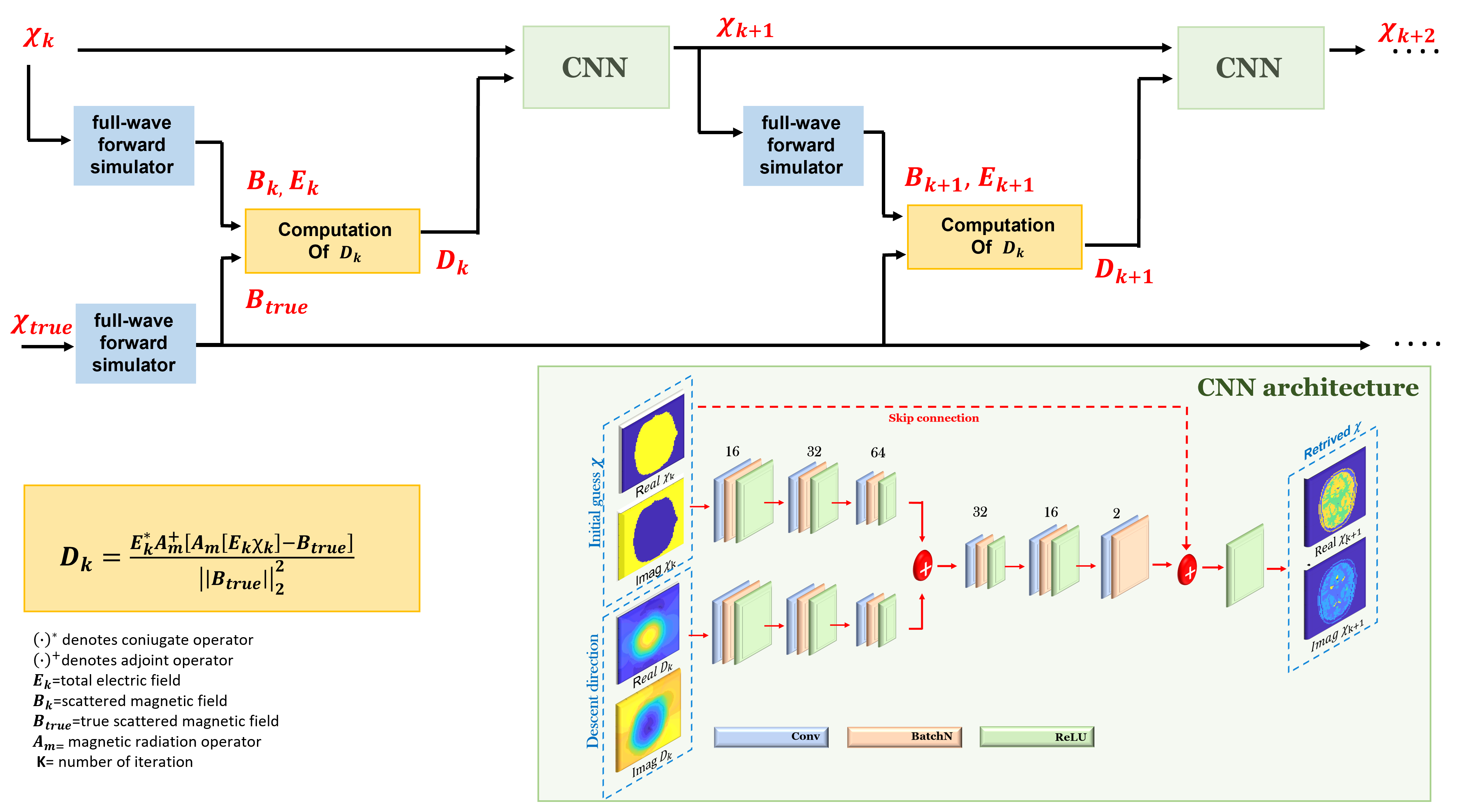
Fig.1. The proposed iterative MR-EPT reconstruction method, which alternates the forward solver operator and the contrast update using CNN. The inputs of the network are the real and imaginary part of the contrast χk and the gradient Dk. The outputs are the real and the imaginary part of the updated contrast χk+1. Note that true=ground-truth.
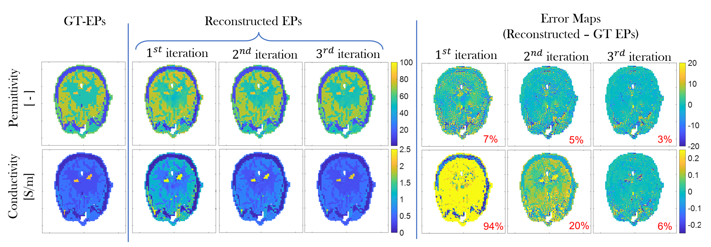
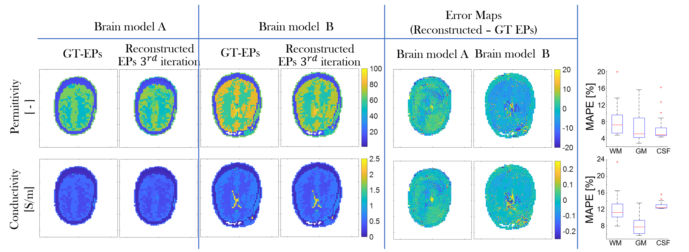
Fig.3. Reconstructed EPs maps(conductivity/permittivity) at the third iteration for two different healthy testing models on the left; error maps (reconstructed EPs – ground-truth EPs) on the right. The MAPE of the reconstructed slices after the three iterations on the right. Also in this figure, boxplots showing the median MAPE (with the 25th-bottom edge and 75th-top edge percentiles), for WM, GM, and CSF EPs reconstructions across all 540 test models are shown
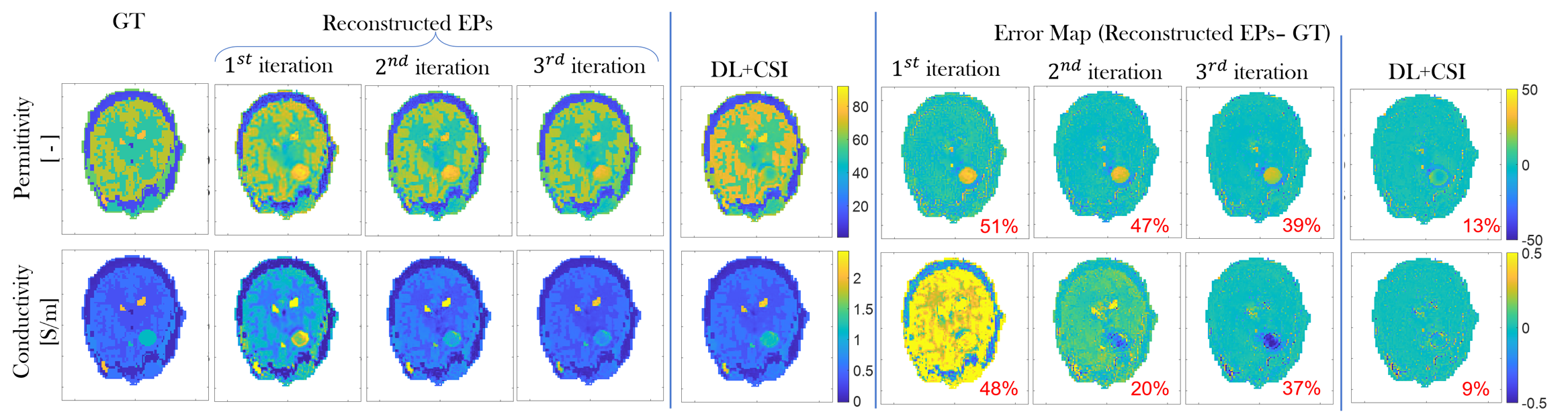
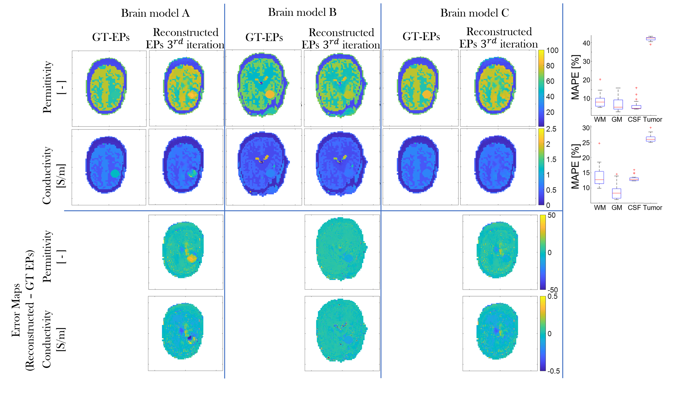
Fig.5. Reconstructed EPs maps (conductivity/permittivity) for different slices of different training models with tumor-like anomalies, after the third iteration, top; error maps (reconstructed EPs – ground-truth EPs), bottom. Also in this figure, boxplots showing the median MAPE (with the 25th-bottom edge and 75th -top edge percentiles), for WM, GM, and CSF EPs reconstructions across all 540 test models with anomalies are shown.