3942
Model Predictive Filtering and Green’s Function Heat Kernel for Real-Time Volumetric MRTI of Laser Interstitial Thermotherapy1Physics and Astronomy, University of Utah, Salt Lake City, UT, United States, 2Department of Radiology and Imaging Sciences, University of Utah, Salt Lake City, UT, United States
Synopsis
Laser interstitial thermotherapy (LITT) is a clinical treatment modality performed under the guidance of magnetic resonance temperature imaging (MRTI). Current limitations in MRTI prevent real-time volumetric monitoring of the tissue regions being treated. In this work, we investigate the use of the model predictive filtering method (MPF), using a Green’s function heat kernel, to reconstruct large field-of-view MRTI data of phantom heating to validate their use for future real-time volumetric MRTI treatment monitoring.
Introduction
Laser interstitial thermotherapy (LITT) is a promising technique for the treatment of a variety diseases.1 Current techniques for magnetic resonance temperature imaging (MRTI) only allow for two-dimensional bi-planar MRTI acquisitions within the clinically appropriate acquisition constraints (~3-6 second temporal resolution, ~1.0x2.0x3.0 mm spatial resolution), which significantly limits the ability of clinicians to fully monitor heating in a three-dimensional tissue volume. The model-predictive filtering method (MPF) has been shown to allow increased field-of-view (FOV) MRTI acquisitions in close-to real time2-3 by supplementing temporally undersampled volumetric data with model-predicted temperature maps. In this work, we propose the use of the computationally efficient Green’s function heat kernel4 to estimate the deposited power density Q and generate accurate temperature predictions to supplement the acquired MRTI data using a brain phantom. This implementation of the MPF algorithm is a step towards real-time, volumetric MRTI measurements of LITT ablative procedures.Methods
Phantom Acquisition: LITT heatings were performed using a laser ablation system (Visualase™, Medtronic) in a gellan gum brain phantom (made in-lab). Five different heatings were repeated in 3 batches, for 15 total heatings. For each batch, “truth” heatings were acquired before and after the heatings to be reconstructed with MPF to ensure that no significant changes occurred in the phantom response to the thermal therapy. A low-power calibration heating was used to obtain the deposited power density Q (watts/m3) using a previously published method based on the Green’s function. Two larger FOV heatings were acquired and reconstructed with MPF. The calibration heating was done with 4 W LITT and all other heatings (“truth” and large FOV) were done with 8 W. MRTI for the truth and calibration heatings had 12 slices with in-plane matrix of 231x217 pixels and 0.9 x 1.8 x 2.5 mm resolution. The two large FOV heatings had 24 and 36 slices, retrospectively, and were subsampled with reduction factors (R) = 2 and R=3, respectively, to achieve the same temporal resolution of 4.5 s. All acquisitions were performed using a segmented EPI sequence (21/12 ms TR/TE, 850 Hz/px bandwidth, 10-degree flip angle, ETL 5, and 4.5 s acquisition time for 12 slices) on a 3T scanner (PrismaFIT, Siemens).MPF/Greens Method: The estimated deposited power density Q was found using the Green’s function heat kernel applied to the 4 W calibration heating. MPF uses the estimated Q together with tissue thermal properties (in this work using literature values; specific heat5, 4186 J/kg/°C, density6, 1030 kg/mm3; thermal conductivity6, 0.560 watts/mm/°C) to predict the temperature map at time point n+1 using Pennes’ bioheat equation7-10, in this work including a model of the LITT probe position and catheter cooling. The predicted temperature map is converted to phase change using the PRF equation, combined with the magnitude image from time point n, and transformed into k-space. In k-space, the MPF-modeled data is combined with the acquired subsampled data for time point n+1 and an updated, large FOV temperature map is calculated.
Results
All reported temperatures were measured as with respect to the baseline (room) temperature of the phantom. Figure 1 shows three orthogonal views of the Q matrix generated by the Green’s function heat kernel. Figure 2 shows 3 orthogonal views of the averaged truth heatings, R=2 and R=3 heatings, and their difference. Figure 3 shows the RMSE in all voxels with ΔT ≥ 6 °C (the point when thermal dose starts to accumulate, assuming 37 °C starting temperature) over time. In Figure 4, the error in voxels ≥ 6 °C and ≥ 17.6 °C (limit when 240CEM43 is delivered during the time of one 4.5 s acquisition) were compared. Figure 5 shows the behavior of the hottest voxel over time for R=2 and R=3.Discussion and Conclusions
The MPF trials with R=2 showed promising accuracy (RMSE of 0.78 °C for voxels at or above 6 °C, Figures 3-5). While some voxels still showed increased error (max error of 1.52 °C and 2.54 dC for 17.6 °C and 6 °C thresholds, respectively), an analysis of the RMSE over time (Figure 3), hottest voxel behavior (Figure 5), and visual analysis of their differences (Figure 2) shows acceptable accuracy, particularly for the dynamics close to the maximum heating when the feedback is of most clinical importance (see time points 9, 10, 11 seconds in Figure 3, 5). Trials with the higher reduction factor R=3 show potential but will require improved strategies to reduce the slightly increased error.The use of the Green’s function heat kernel in conjunction with the MPF algorithm showed encouraging accuracy for volumetric MRTI monitoring of LITT procedures. These procedures could easily be applied within the computational constraints required for clinical real-time volumetric monitoring.
Acknowledgements
Authors acknowledge support from the Mark H. Huntsman endowed chair and NIH grants R01EB028316, R03EB029204, S10OD026788 and S10OD018482.References
1. Chen, Clark et al. “Laser interstitial thermotherapy (LITT) for the treatment of tumors of the brain and spine: a brief review.” Journal of neuro-oncology vol. 151,3 (2021): 429-442. doi:10.1007/s11060-020-03652-z
2. Todd, Nick et al. “Model predictive filtering for improved temporal resolution in MRI temperature imaging.” Magnetic resonance in medicine vol. 63,5 (2010): 1269-79. doi:10.1002/mrm.22321
3. Odéen, Henrik et al. “MR thermometry for focused ultrasound monitoring utilizing model predictive filtering and ultrasound beam modeling.” Journal of therapeutic ultrasound vol. 4 23. 22 Sep. 2016, doi:10.1186/s40349-016-0067-6
4. Freeman, N. J., Odéen, H., & Parker, D. L. (2018). 3D-specific absorption rate estimation from high-intensity focused ultrasound sonications using the Green's function heat kernel. Medical physics, 45(7), 3109–3119. https://doi.org/10.1002/mp.12978
5. Cahto, J.C. and Lee, R.C. (1998), The Future of Biothermal Engineering. Annals of the New York Academy of Sciences, 858: 1-20. https://doi.org/10.1111/j.1749-6632.1998.tb10135.x
6. R. L. King, Y. Liu, S. Maruvada, B. A. Herman, K. A. Wear and G. R. Harris, "Development and characterization of a tissue-mimicking material for high-intensity focused ultrasound," in IEEE Transactions on Ultrasonics, Ferroelectrics, and Frequency Control, vol. 58, no. 7, pp. 1397-1405, July 2011, doi: 10.1109/TUFFC.2011.1959.
7. Rawnsley, R. J., Roemer, R. B., & Dutton, A. W. (1994). The simulation of discrete vessel effects in experimental hyperthermia. Journal of biomechanical engineering, 116(3), 256–262. https://doi.org/10.1115/1.2895728
8. Moros, E. G., Dutton, A. W., Roemer, R. B., Burton, M., & Hynynen, K. (1993). Experimental evaluation of two simple thermal models using hyperthermia in muscle in vivo. International journal of hyperthermia : the official journal of European Society for Hyperthermic Oncology, North American Hyperthermia Group, 9(4), 581–598. https://doi.org/10.3109/02656739309005054
9. Roemer R. (1998), Thermal dosimetry and treatment planning. In: Gautherie M, editor. Thermal dosimetry. Berlin: Springer. p 119–214.
10. Pennes H. H. (1998). Analysis of tissue and arterial blood temperatures in the resting human forearm. 1948. Journal of applied physiology (Bethesda, Md. : 1985), 85(1), 5–34. https://doi.org/10.1152/jappl.1998.85.1.5
Figures
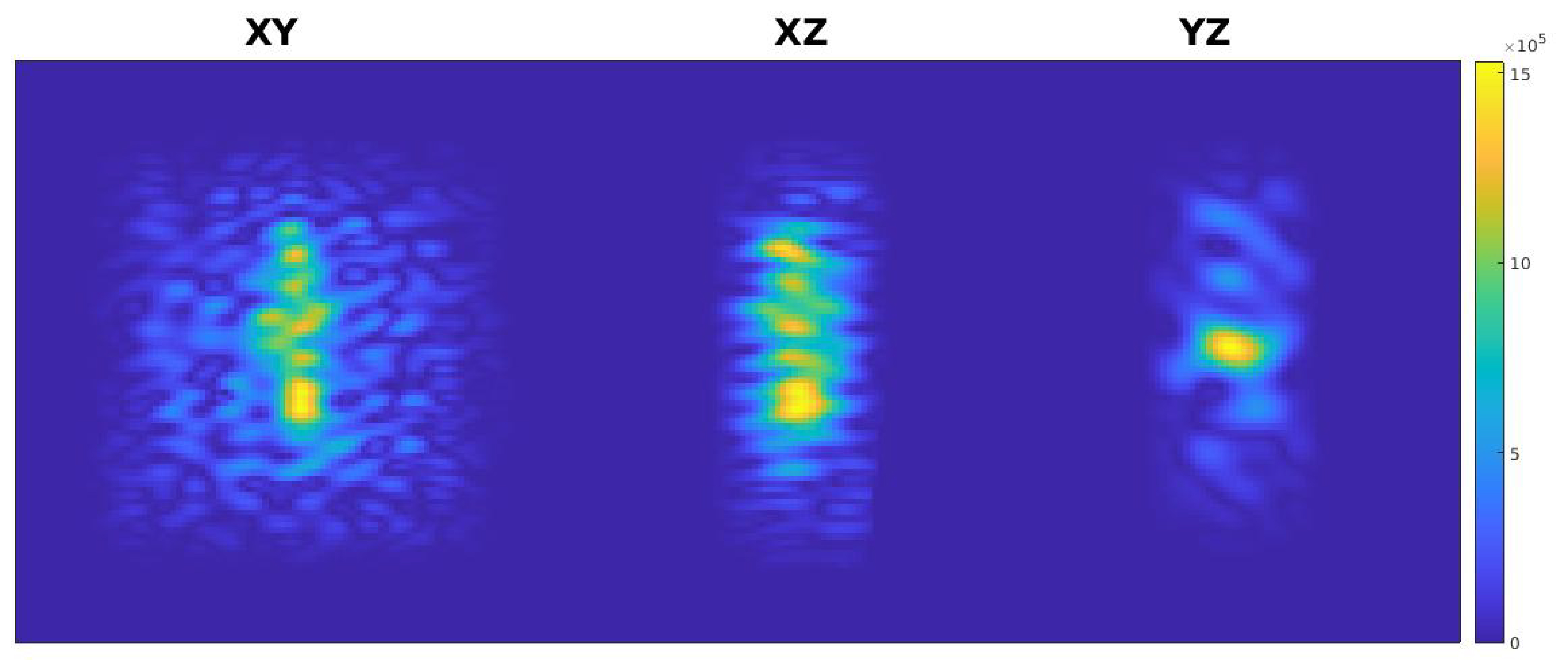
Figure 1: Three orthogonal views of the Q pattern derived from the Green’s function heat kernel and one 4 W calibration heating, obtained from the first heating dynamic and later scaled for application to the 8 W trials. A 3D Tukey filter was applied to reduce noise outside of the region including the heating. Noise artifacts are likely the result of the calibration MRTI noise. Colorbar is in W/m3.
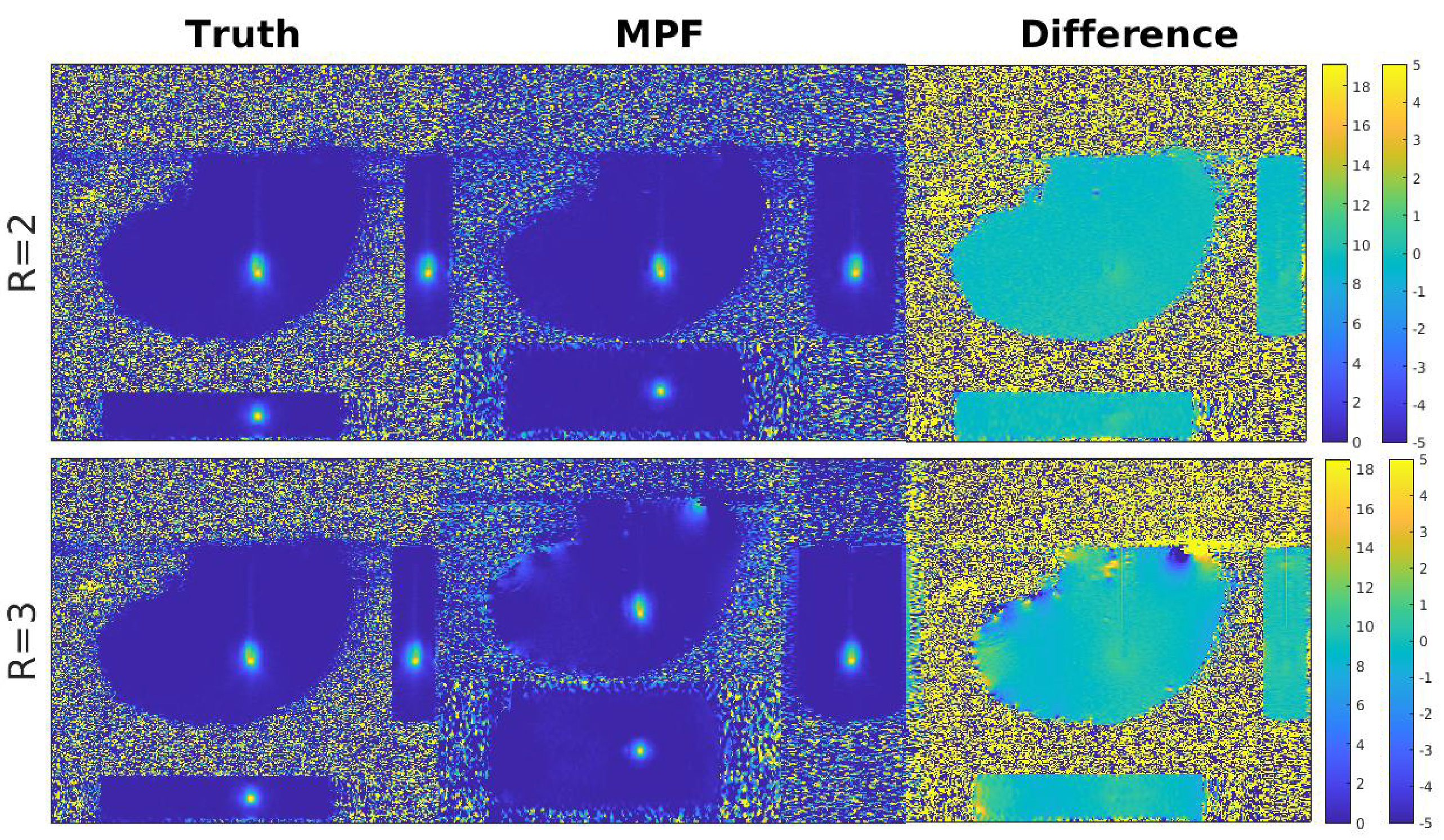
Figure 2: Three orthogonal views at the hottest time point of the averaged “truth” data, MPF data and their difference are shown (left to right, respectively) for both R=2 (top) and R=3 (bottom) reduction factors. Note the larger FOV in the slice direction for MPF compared to “truth”. Minor differences can be observed near the edges of the heating patterns in the difference image. Colorbars (left for “truth” and MPF, right for difference image) are in °C.
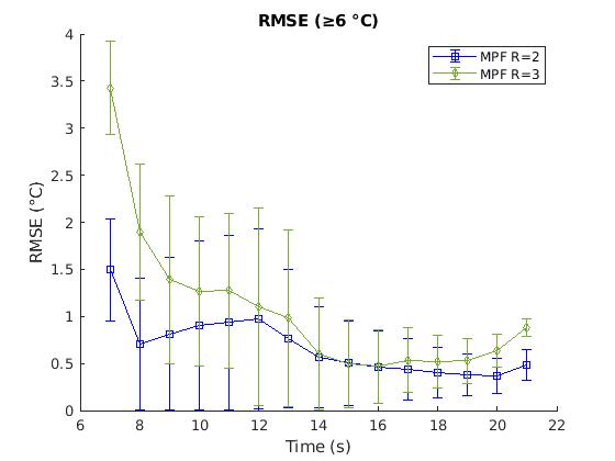
Figure 3: The RMSE (in °C) and standard deviation for the three repeated heatings at each R are shown for all voxels at or above 6 °C.
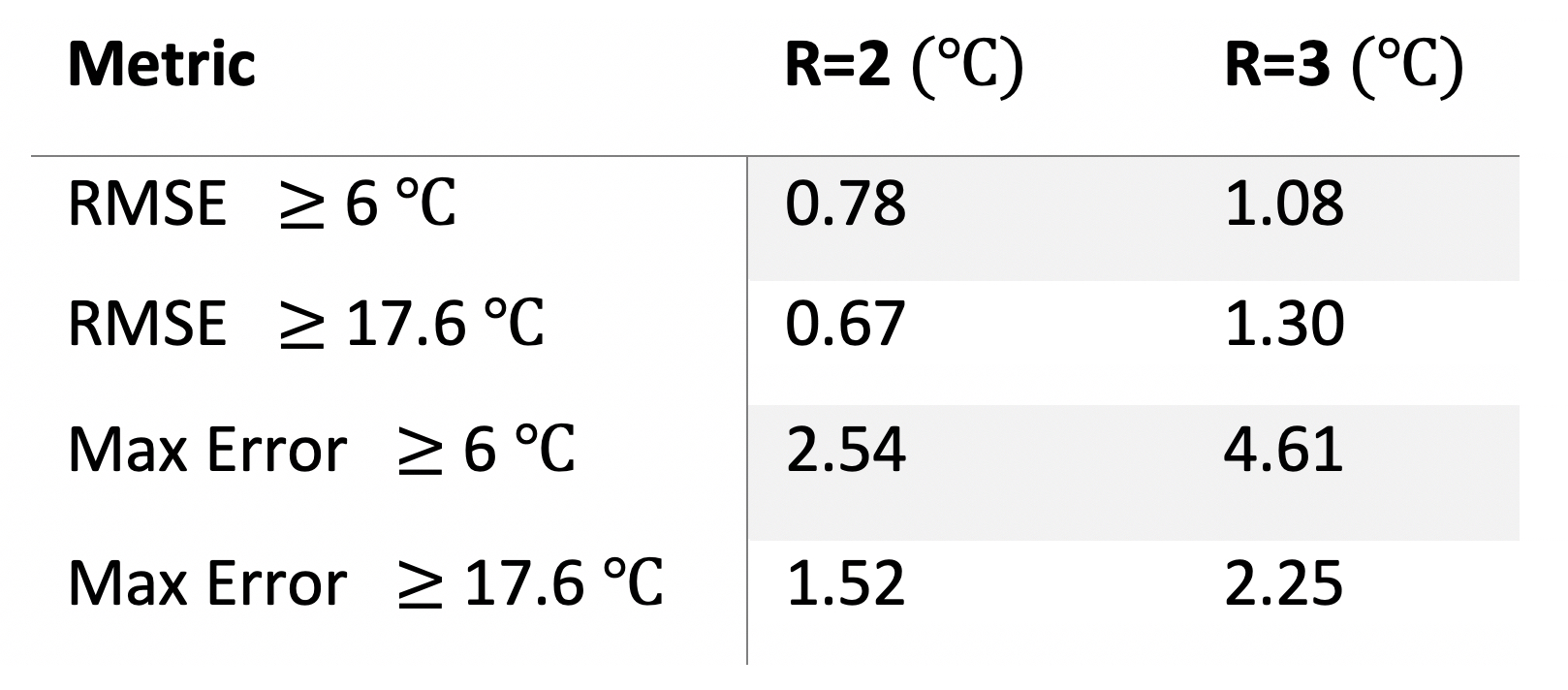
Figure 4: RMSE and maximum error (in °C) for all voxels at or above 6 °C and 17.6 °C for the three repeated heatings at each R.
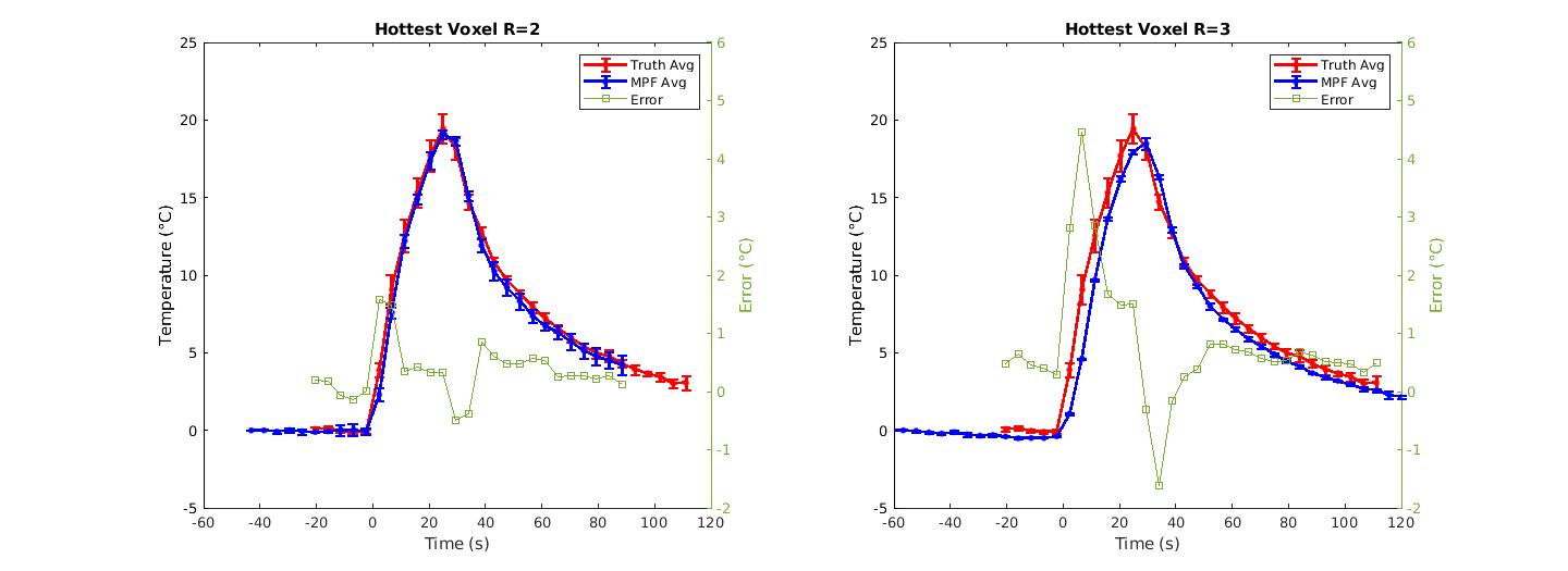
Figure 5: Mean +/- standard deviation of the the hottest voxel over time for the three repeated heatings reconstructed with R=2 and R=3 compared to the hottest voxel in the repeated “truth” data. The difference at each time point ( °C) is shown in green using the axis to the right.