3819
Acceleration of Relaxation Time Mapping by Joint K-space and Image-space Parallel Imaging (KIPI)1Key Laboratory for Biomedical Engineering of Ministry of Education, Department of Biomedical Engineering, College of Biomedical Engineering & Instrument Science, Zhejiang University, Hangzhou, China, 2MR Collaboration, Siemens Healthcare Ltd., Shanghai, China, 3Department of Neurology, The First Affiliated Hospital, Zhejiang University, Hangzhou, China, 4Cancer Center, Zhejiang University, Hangzhou, China
Synopsis
The relaxation time mapping has proven to be an important diagnostic tool, but it is limited by the prolonged scan time due to the measurements of multiple frames at the same location. In this study, the recently proposed auto-calibrated reconstruction method by joint k-space and image-space parallel imaging (KIPI) is utilized for the acceleration of relaxation time mapping. Combined with the ESPIRiT method, KIPI generates improved coil sensitivity maps and allows an acceleration factor of up to 4-fold for acquiring source images, yielding the accurate parameter map without obvious errors or artifacts.
Introduction
The relaxation time mapping, which can characterize intrinsic tissue-dependent information, has proven to be a valuable diagnostic tool(1-3). However, the long scan times imposed by conventional methods limit its routine clinical application since multiple images with modulated sequence parameters are required(4). Recently, an auto-calibrated reconstruction method by joint k-space and image-space parallel imaging (KIPI) was proposed to accelerate the CEST acquisition(5). Here, we modify the KIPI method by combining the ESPIRiT(6) approach to accelerate the relaxation time mapping.Theory
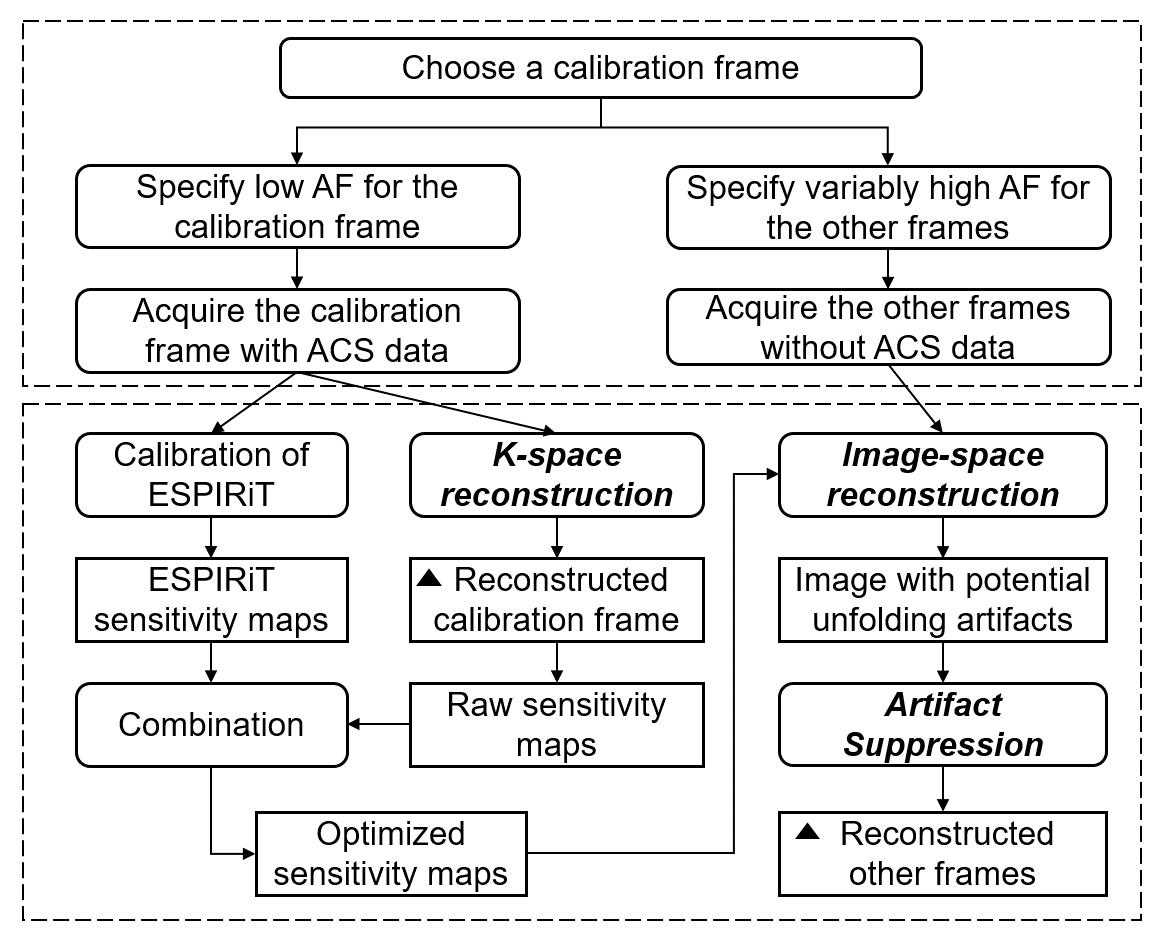
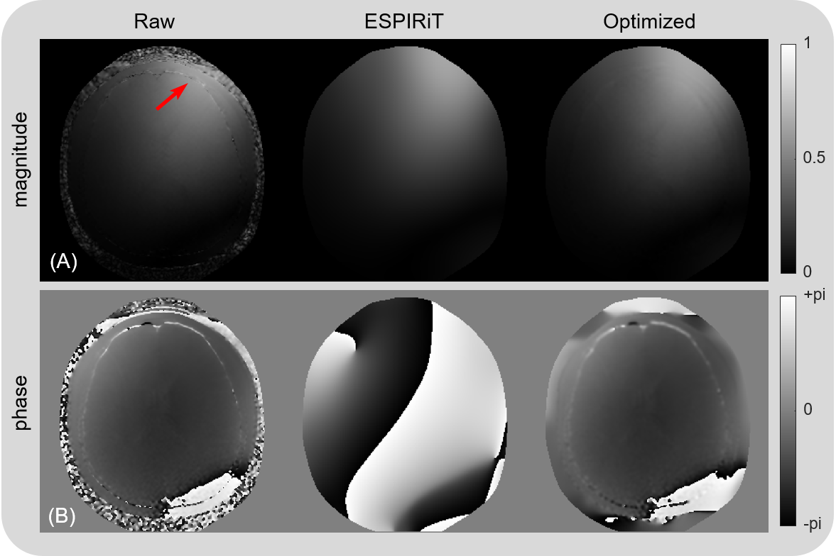
In relaxation time mapping, the dataset comprises a series of images acquired with different pulse sequence parameters from the same volume(4), which implies that the coil sensitivity maps of different frames are essentially the same. The conventional SENSE(7) method uses sensitivity maps explicitly from a separate reference scan, while the GRAPPA(8) method utilizes sensitivity encoding implicitly via correlations in k-space estimated from autocalibration signals (ACS). However, it is difficult to obtain accurate sensitivity maps for SENSE reconstruction, limiting its maximum achievable acceleration factor in practice. As for GRAPAA, the ACS data needs to be repetitively acquired for all relaxation time mapping frames, causing a substantial overhead scan time.The recently-proposed KIPI(5) method utilizes variable acceleration factors for different CEST frames and incorporates the advantages of both SENSE and GRAPPA. KIPI requires a CEST frame to be sampled at a low acceleration factor (e.g. AF=2), uses GRAPPA to fill the unsampled k-space, obtains sensitivity maps from GRAPPA-generated full k-space, and then reconstructs the other highly-undersampled (AF>2) frames with SENSE and the artifact suppression algorithm(9). However, when applying KIPI to inversion recovery (IR) relaxation time mapping sequences, the sensitivity maps obtained by dividing the sum-of-squares (SOS) image into the image from each channel are not always accurate, especially at the scalp area. In this work, the optimized sensitivity maps are obtained by combining the raw and ESPIRiT(6) sensitivity maps, with the reconstruction flowchart shown in Fig. 1.
Methods
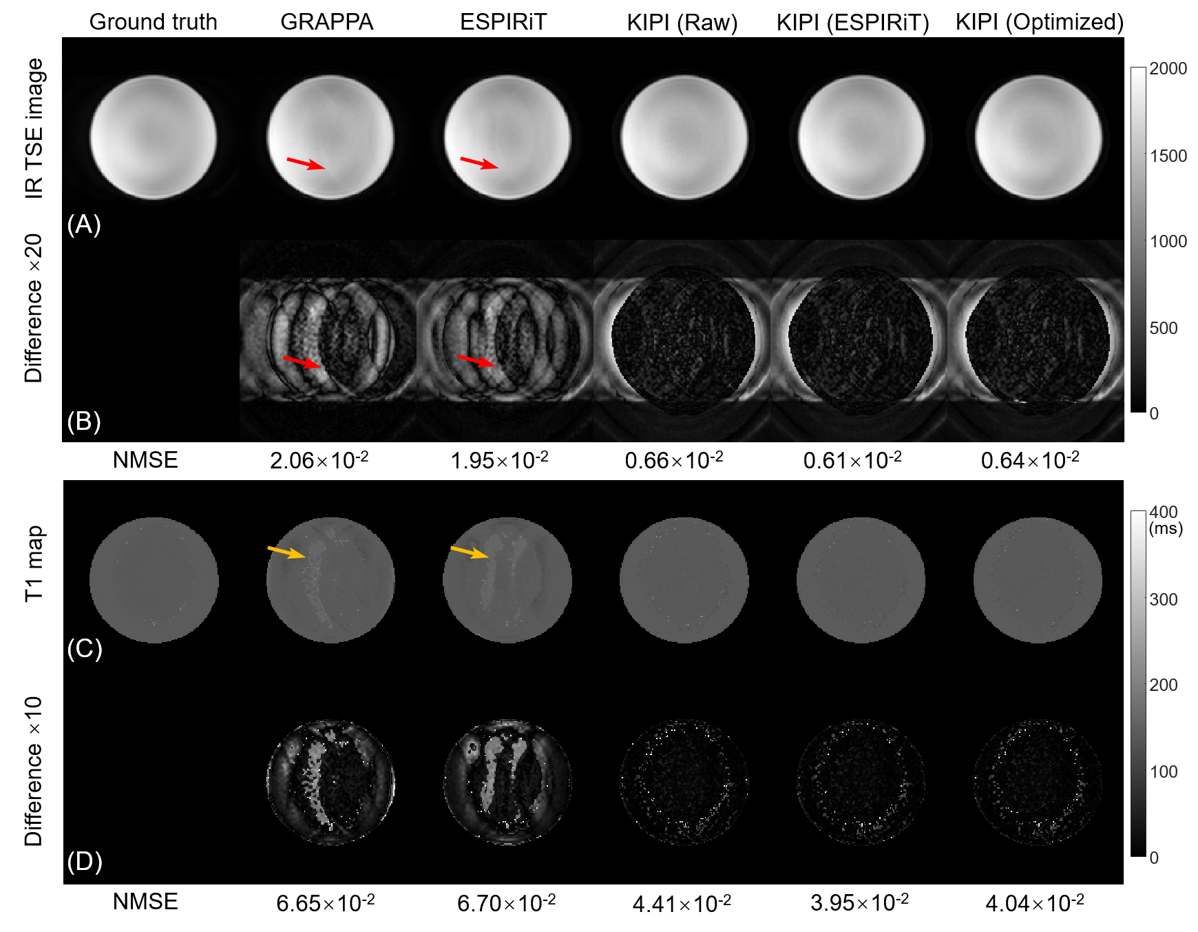
Human and phantom experiments were conducted on a 3T Siemens Prisma MRI system with a multi-channel receiver. An IR TSE sequence was running for T1 mapping with full k-space sampling, and time of inversion (TI) = 50, 150, 300, 500, 800, 1300, and 2000ms. For retrospective undersampling, the TI=2000ms frame was selected as the calibration frame with AF=2 and 24 ACS lines for KIPI to generate the sensitivity maps and correction maps. And the remaining six IR frames were undersampled with AF=4 and without ACS data.For KIPI reconstruction, the k-space of the AF=2 calibration frame was firstly refilled by GRAPPA, from which the raw sensitivity maps were calculated by dividing the SOS image into each channel image. The ESPIRiT sensitivity maps were derived from the ACS data of the calibration frame. The values in the noise region of the raw sensitivity map were replaced by those of the ESPIRiT sensitivity, which was defined as less than 10% of the maximum signal intensity. Then a locally-weighted polynomial regression(7) was implemented to fit the combined sensitivities to get the optimized sensitivity maps (Fig. 2). Besides, the phase of the sensitivity map was generated individually due to the gap between raw and ESPIRiT maps. With the optimized sensitivity maps, KIPI reconstructed the other AF=4 frames by SENSE with artifact suppression(5,9).
For comparison, the regular GRAPPA and ESPIRiT reconstruction were implemented which used the same data as the KIPI method. Moreover, KIPI was executed with three sensitivity maps as shown in Fig. 2 while other conditions were kept the same.
Results
Figure 2 shows three kinds of sensitivity maps from a healthy volunteer in one coil channel. The raw sensitivity map has a noisy edge and unsmooth jump(red arrow), while the ESPIRiT one is very smooth but a little blurry. The optimized sensitivity map retains the details and avoids the interference of noise, and its phase map has a high agreement with the raw one.Figure 3 displays the reconstructed phantom images and the corresponding T1 maps from undersampled IR TSE data. For all three schemes of sensitivity maps, KIPI obtains results with high quality, while GRAPPA and ESPiRiT yield obvious artifacts in both source images (red arrows) and T1 maps (yellow arrows).
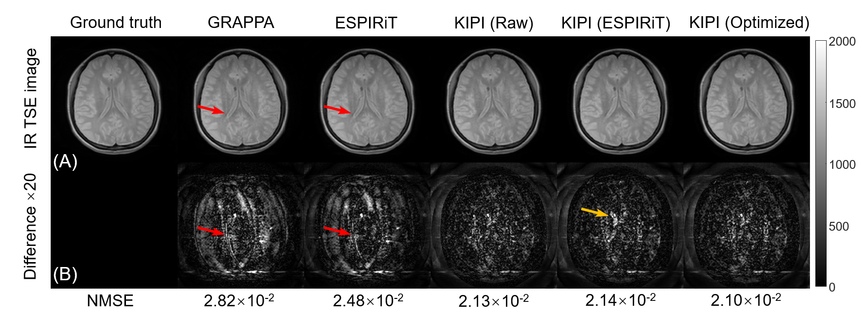
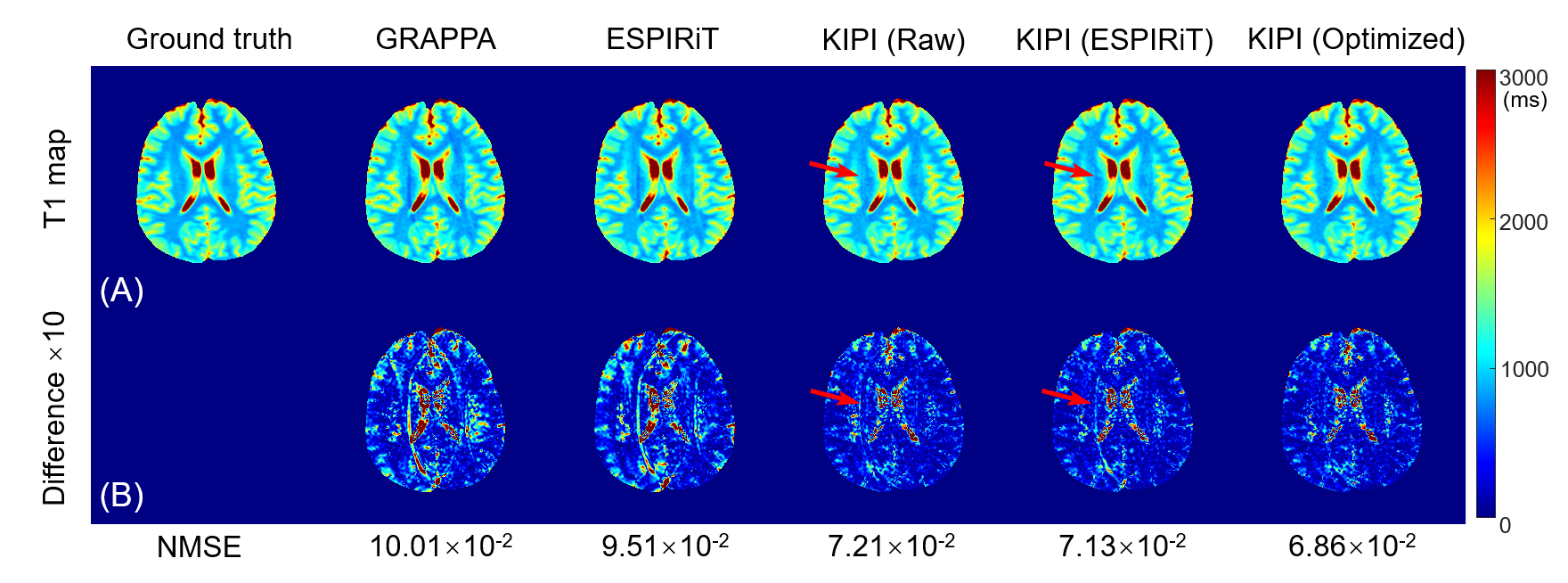
Figure 4 shows the TI=50ms frame reconstructed by GRAPPA, ESPIRiT, and KIPI. The results of GRAPPA and ESPIRiT have evident unfolding artifacts, indicated by the red arrows, which are absent in KIPI results. Figure 5 displays the T1 maps calculated from the source images of Figure 4. Noticeable artifacts can be seen in the results reconstructed by GRAPPA and ESPIRiT while the KIPI method generates T1 maps that are more consistent with the ground truth. The KIPI reconstruction with optimized sensitivity maps shows the best results among all three kinds of sensitivity maps.
Conclusion
KIPI is a novel and non-iterative auto-calibrated reconstruction method that integrates the strength of both k-space and image-space parallel imaging. Combining the ESPIRiT method, KIPI generates more accurate and robust sensitivity maps. KIPI allowed an acceleration factor of up to 4-fold for 2D relaxation time mapping, essentially without compromising the image quality. The advantages of KIPI may be exploited to accelerate other MR parameter mapping that acquires multiple image frames at the same location.Acknowledgements
NSFC grant numbers: 61801421 and 81971605. Leading Innovation and Entrepreneurship Team of Zhejiang Province: 2020R01003. This work was supported by the MOE Frontier Science Center for Brain Science & Brain-Machine Integration, Zhejiang University.References
1. Bottomley PA, Hardy CJ, Argersinger RE, Allenmoore G. A REVIEW OF H-1 NUCLEAR-MAGNETIC-RESONANCE RELAXATION IN PATHOLOGY - ARE T1 AND T2 DIAGNOSTIC. Medical Physics 1987;14(1):1-37.
2. Mackay A, Whittall K, Adler J, Li D, Paty D, Graeb D. IN-VIVO VISUALIZATION OF MYELIN WATER IN BRAIN BY MAGNETIC-RESONANCE. Magnetic Resonance in Medicine 1994;31(6):673-677.
3. Sibley CT, Noureldin RA, Gai N, Nacif MS, Liu S, Turkbey EB, Mudd JO, van der Geest RJ, Lima JAC, Halushka MK, Bluemke DA. T1 Mapping in Cardiomyopathy at Cardiac MR: Comparison with Endomyocardial Biopsy. Radiology 2012;265(3):724-732.
4. Crawley AP, Henkelman RM. A COMPARISON OF ONE-SHOT AND RECOVERY METHODS IN T1-IMAGING. Magnetic Resonance in Medicine 1988;7(1):23-34.
5. Zu T, Sun Y, Wu D, Zhang Y. Accelerated Chemical Exchange Saturation Transfer Acquisition by Joint K-space and Image-space Parallel Imaging (KIPI). Proceedings of the 29th Annual Metting of ISMRM 2021:2598.
6. Uecker M, Lai P, Murphy MJ, Virtue P, Elad M, Pauly JM, Vasanawala SS, Lustig M. ESPIRiT-an eigenvalue approach to autocalibrating parallel MRI: Where SENSE meets GRAPPA. Magnetic Resonance in Medicine 2014;71(3):990-1001.
7. Pruessmann KP, Weiger M, Scheidegger MB, Boesiger P. SENSE: Sensitivity encoding for fast MRI. Magnetic Resonance in Medicine 1999;42(5):952-962.
8. Griswold MA, Jakob PM, Heidemann RM, Nittka M, Jellus V, Wang J, Kiefer B, Haase A. Generalized autocalibrating partially parallel acquisitions (GRAPPA). Magnetic Resonance in Medicine 2002;47(6):1202-1210.
9. Zhang Y, Heo H-Y, Jiang S, Zhou J, Bottomley PA. Fast 3D chemical exchange saturation transfer imaging with variably-accelerated sensitivity encoding (vSENSE). Magnetic Resonance in Medicine 2019;82(6):2046-2061.
Figures