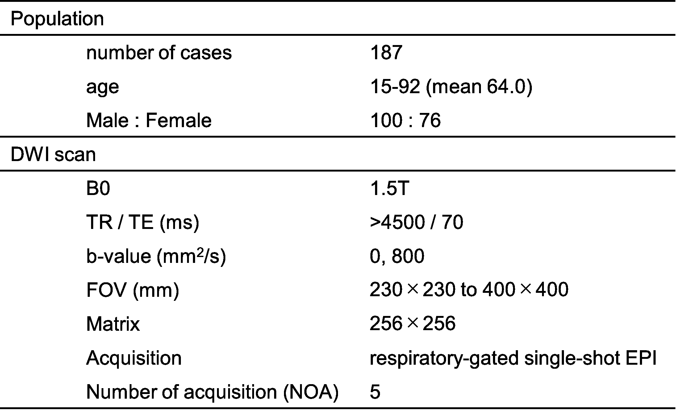
3809
The usefulness of 4D convolution in deep-learning-based noise reduction for low-SNR body DWI1National institutes for Quantum science and Technology, Chiba, Japan
Synopsis
Deep-learning-based slice-by-slice noise reduction may not be suitable for low-SNR body DWI that contains insufficient information in the original single slice. Moreover, averaging multiple acquisitions after denoising to avoid this problem is insufficient because it causes blurring owing to a mismatch between acquisitions. Herein, we designed a neural network that utilises 4D convolution to incorporate adjacent slices and multiple acquisitions simultaneously for a slice to achieve adequate denoising. The results support the utility of the proposed method in comparison with the usual slice-by-slice method and averaging.
Introduction
Many reports have addressed deep-learning-based noise removal1-3, but most of them are simple slice-by-slice 2D image transformations, such as converting a slice image without averaging (number of acquisitions=1 [NOA1]) to an image-equivalent of an image obtained by averaging multiple acquisitions.However, in a body diffusion-weighted image (DWI) with low signal-to-noise ratio (SNR), it is not difficult to apply this method directly because NOA1 often has insufficient information to reconstruct the appropriate image. This problem may be solved by using more than one acquisition for the input; however, such images tend to appear smoothened because of the motion-related-mismatch between acquisitions, which eventually blurs the small structures. In this study, we developed a neural network that utilizes 4D convolution to denoise the input image series. The concept was to incorporate all relevant information for each pixel, including the neighboring pixels in 3D (i.e. including the adjacent slices), and the same 3D area in another acquisition, instead of referring to only the neighboring pixels in the same slice in the same acquisition as done for the usual 2D convolution.
This study aimed to evaluate the usefulness of this novel strategy.
Methods
A total of 187 cases that included body DWI scans as part of the tumor screening, were extracted from the clinical database. The subject population and major DWI scanning parameters are summarized in Figure 1.The outline of the proposed network is shown in Figure 2. The task given to this network was to estimate NOA5 as denoised images from the NOA2 equivalent data input that was derived from the original NOA5. The proposed network was designed to accept three adjacent slices and two acquisitions simultaneously and applied both 4D and 2D convolutions in combination. The control network (Figure 3) had a design similar to that of the proposed network, except that it accepted each slice and acquisition as separate inputs, and the results of different acquisitions were averaged at the end. Therefore, all convolutions were performed in 2D.
The subjects were randomly divided into 99 training and 38 testing cases. The networks were trained using the training cases: optimiser = Adam4 (lr=0.001, beta=0.5), epoch=50, and loss= mean absolute error. The Chainer5 platform was used for all deep-learning procedures.
The trained networks were tested using test cases. The denoised series obtained via the proposed network (4D-conv), control network (2D-conv), and NOA2 were compared both visually and numerically. For numerical comparisons, the mean absolute difference (MAE) and structural similarity index measure for DWI (b=800) were obtained for each case in comparison with NOA5 (MAEDWI and SSIM). In addition, ADC maps were calculated for 4D-conv, 2D-conv, and NOA2, and MAE were obtained similarly (MAEADC). All indices were statistically compared between the noise-reduction methods using the Wilcoxon signed-rank test (P<.05 was considered significant).
Results
Examples of the denoised images are shown in Figure 4. Visually, the appearance of 4D-conv was closer to NOA5 compared to 2D-conv and NOA2.The results of the statistical comparisons are shown in Figures 5. The MAEDWI was significantly smaller in 4D-conv and 2D-conv than in NOA2 (P<.001), but the difference between 4D-conv and 2D-conv was not significant (P=0.56). The SSIM was significantly higher, and MAEADC was significantly smaller in 4D-conv than in 2D-conv and NOA2 (P<.001). However, the SSIM was significantly lower, and MAEADC was significantly higher in 2D-conv than in NOA2 (P<.001).
Discussion
In this study, we proposed a new neural network to adequately reduce noise from NOA2 input in low-SNR body DWI. The major underlying concept was to utilize 4D convolution to incorporate all relevant information for calculating the output value for a certain pixel. However, repeating many 4D convolutions was difficult because of the enormous memory consumption involved, and was applied only once to create the output. Instead, the pathway including repeated 2D convolutions with softmax activation at the end was merged with this layer so that the large optimized receptive field would be available, similar to our previous study6.4D-conv could not decrease MAEDWI compared to 2D-conv, but successfully increased the SSIM. This could be because the proposed strategy was better in optimizing the convolution to fit the specific situation for each pixel, and thus the blurring was suppressed well. Furthermore, the fact that MAEADC was significantly smaller in 4D-conv compared to 2D-conv and NOA2 suggests that 4D-conv did not only make the DWI appearance closer to NOA5 but was appropriate to preserve the underlying diffusion information. However, the low SSIM and high MAEADC in 2D-conv supports the issue described in the introduction that blurring may occur when such a method is used.As a limitation, this study only focused on the overall image quality and did not evaluate the 4D-conv’s ability to delineate individual lesions.
Conclusion
The proposed method using 4D convolution may be useful for denoising body DWI with low SNR because it can denoise images adequately without blurring.Acknowledgements
This research was supported by a Grant-in-Aid for Scientific Research (Kakenhi #17K10385) from the Japan Society for the Promotion of Science (JSPS), and by QST President’s Strategic Grant QST Advanced Study Laboratory.References
1. Kidoh, M., Shinoda, K., Kitajima, M., et al. Deep Learning Based Noise Reduction for Brain MR Imaging: Tests on Phantoms and Healthy Volunteers (2020) Magn Reson Med Sci. 19:195-206
2. Jose V. Manjon and Pierrick Coupe. MRI denoising using Deep Learning and Non-local averaging. (2019) arXiv:1911.04798 (https://arxiv.org/abs/1911.04798) [accessed Nov.10, 2021]
3. Koonjoo, N., Zhu, B., Bagnall, G. Cody, et al. Boosting the signal-to-noise of low-field MRI with deep learning image reconstruction. (2021) Sci Rep. 11:8248
4. Diederik P. Kingma and Jimmy Ba. Adam: A Method for Stochastic Optimization (2014) arXiv:1412.6980 (https://arxiv.org/abs/1412.6980) [accessed Nov.10, 2021]
5. Tokui, S., Okuta, R., Akiba, T., et al. Chainer: A Deep Learning Framework for Accelerating the Research Cycle. (2019) arXiv:1908.00213 (https://arxiv.org/abs/1908.00213) [accessed Nov.10, 2021]
6. Nozaki, H., Tachibana, Y., Otsuka, Y., et al. Deep learning-based DWI Denoising method that suppressed the "instability" problem. (2021) Proceedings of ISMRM 2021 #2442.
Figures
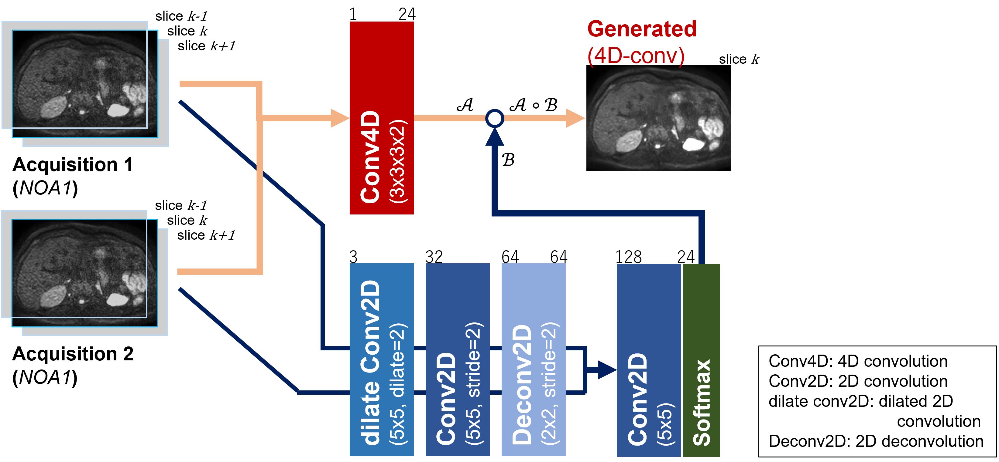
The outline of the proposed neural network. The network accepts input of three slices each (the target and the adjacent slices) from the two acquisitions and processes them simultaneously. The numbers in brackets are the kernel size and the value of dilation and stride factors if they were not 1. The small numbers at the shoulder of the layers are the number of input / output channels.
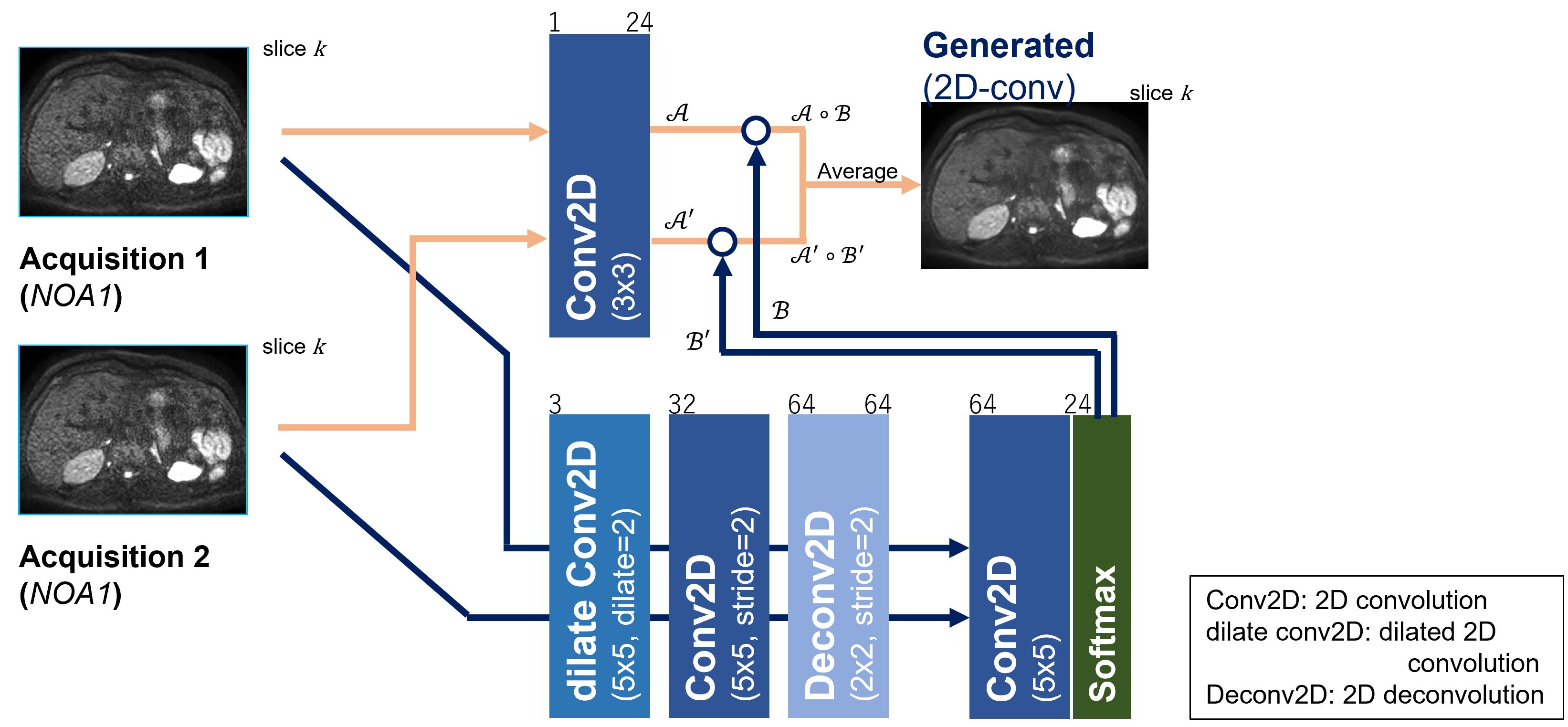
The outline of the control neural network. The basic structure was similar to that of the proposed model (see Figure 2), except that the process was performed slice by slice, therefore all the convolutions were in 2D.
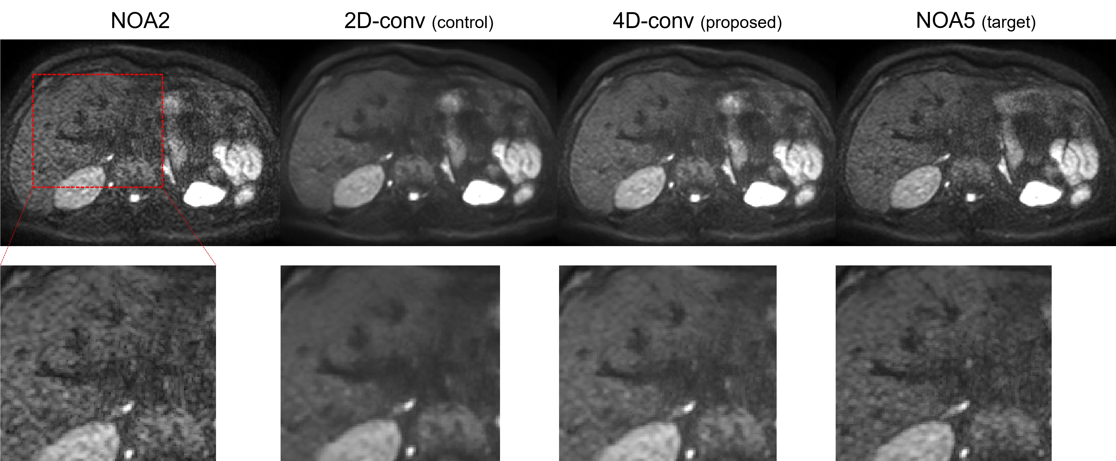
The example images of NOA2, 2D-conv, 4D-conv, and NOA5. Visually, the appearance of 4D-conv was closer to NOA5 compared to 2D-conv and NOA2. On the other hand, the 2D-conv seemed to have the least noise, but also most "smoothed".
NOA2: averaging 2 acquisitions as usual, 2D-conv: generated image using the control network, 4D-conv: generated image using the proposed network, NOA5: averaging 5 acquisitions (the target image).
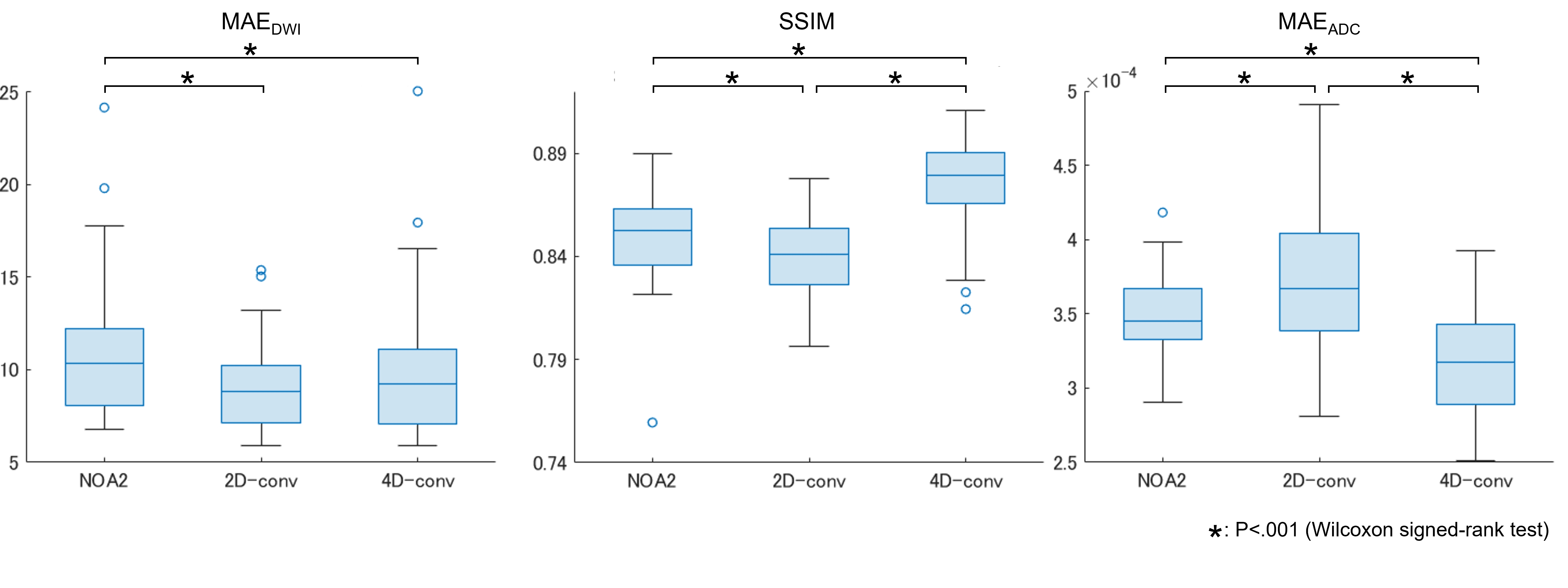
The results of statistical comparisons. The 4D-conv achieved better results with significant differences for all indices compared to NOA2, and for all except MAEDWI (no significant difference) compared to 2D-conv. The 2D-conv was worse than NOA2 in ISMM and MAEADC with significant differences.
MAE: mean absolute error, SSIM: structural similarity index measure, MAEDWI and MAEADC: MAE obtained for DWI (b=800) and ADC map, NOA2: averaging 2 acquisitions as usual, 2D-conv: generated image using the control network, 4D-conv: generated image using the proposed network