3633
Towards fast and precise tissue conductivity imaging in brain
Jun Cao1,2, Iain Ball3, and Caroline Rae1,2
1Neuroscience Research Australia, Sydney, Australia, 2School of Medical Sciences, University of New South Wales, Sydney, Australia, 3Philips Australia & New Zealand, Sydney, Australia
1Neuroscience Research Australia, Sydney, Australia, 2School of Medical Sciences, University of New South Wales, Sydney, Australia, 3Philips Australia & New Zealand, Sydney, Australia
Synopsis
Here we tested the boundaries of the speed and precision of phase MREPT in brain using balanced FFE. Baseline maps with conductivity variance of < 5% could be safely accelerated with compressed SENSE 6 without sacrifice of precision, and scans acquired as quickly as 1.89 s. Precision could be further improved by whole head B1 mapping. MREPT mapping should be conducted task free for best results.
Introduction
Electric properties of tissue including conductivity and permittivity can provide auxiliary information for disease diagnosis and monitoring. Magnetic resonance electric properties tomography (MREPT) is emerging as a noninvasive imaging method for mapping tissue electric properties.1,2 Phase-MREPT using the phase map may be particularly useful for clinical applications.3,4 Implementation of MREPT in the clinic requires a robust and reliable method and a short scan time. This could be accomplished using Compressed SENSE but the effect of this on the precision and reliability of the calculated variables is unknown. Here, we investigated the impact of increased Compressed SENSE (CS) factors on the reliability of conductivity values. We investigated the effect of field mapping on measurement precision as well as the impact of brain activity, such as video watching on tissue conductivity values.5Methods
Data acquisitionReliability was tested by scanning five healthy subjects (Age: 35.8 ± 8.5, two females, three males) at 3T (Ingenia CX, Philips Healthcare, Best, The Netherlands) on two separate sessions (different days, similar time of day). Parameters: BFFE, TR/TE = 3.2/1.6 ms, nonselective RF pulses, flip angle 25° , resolution 1.3×1.3×1 mm3, sagittal slices.
Utility of compressed SENSE was tested by scanning additional five healthy subjects (Age: 32.2 ± 12.3, three females, two males) using the BFFE approach above, with increasing CS factors. The default CS factor used for reference was 1.3. Conductivity maps were calculated using CS factors from 2 to 12, and error maps were obtained by subtracting these conductivity maps from the reference. The reference scan duration was 4 min 33 s.
A fast acquisition (dynamic scan time 1.89 s) was tested by scanning one healthy subject (Age: 30, male) using BFFE with CS factor 4. Parameters: BFFE, TR/TE = 1.58/0.79 ms, nonselective RF pulses, flip angle 25° , resolution 3×3×3 mm3, sagittal slices, 520 dynamics.
Comparisons of B1 mapping methods were tested by scanning four healthy subjects (Age: 40.3 ± 11.1, one female, three males) at 3T. Two bFFE scans were acquired for each B1 mapping method, including single-slice 2D DREAM, full coverage DREAM and full coverage dual TR. Parameters: BFFE, TR/TE = 2.5/1.25 ms, nonselective RF pulses, flip angle 25° , sagittal slices, acquired resolution 1.3×1.3×1 mm3 reconstructed to 1×1×1 mm3.
Effect of video watching was tested by scanning additional four healthy subjects (Age: 42.0 ± 15.1, two females, two males) using BFFE with or without video watching during scanning. Parameters: BFFE, TR/TE = 2.5/1.25 ms, nonselective RF pulses, flip angle 25° , sagittal slices, acquired resolution 1.3×1.3×1 mm3 reconstructed to 1×1×1 mm3.
3D T1 TFE scans were acquired from each subject for anatomical reference. Parameters: 190 slices (R-L) in the sagittal acquisition plane, 240 mm FOV, 1x1x1 mm3 acquired voxel size, non-selective excitation, TE/TR/TI = 7.25/3.42/850 ms, flip angle 8° with a TFE factor = 117 and TFE shot interval = 2000 ms.
Data analysis
T1W images were co-registered to bFFE images for segmenting brain into white matter, gray matter and CSF by FSL to alleviate boundary artifacts in the calculation. An average parabolic phase fitting method was used to reduce artifacts amplified in the Laplacian.6 For each dimension of a voxel, parabolic fitting was conducted on both sides of the voxel. The average of second derivatives of the two quadratic expressions was assigned to the second derivative of the target phase in this dimension.
Results
Figure 1 shows conductivity values of white matter, gray matter and CSF of five healthy subjects in two separate sessions. The measured conductivity values of white matter, gray matter and CSF at 3T Larmor frequency (127.78 MHz) were 0.42 ± 0.02, 0.63 ± 0.03, 2.24 ± 0.10 S/m. Figure 2 shows the variation conductivity of white matter, gray matter and CSF with increasing CS factors. White matter conductivity showed minimal deviation with CS factors up to 5 with deviations increasing at CS factors > 6. The conductivity of gray matter showed minimal deviation up to CS factor 6 with increasing deviation at CS factor >8. The ultra fast BFFE with dynamic 1.89 s also showed good precision with coefficient of variances over the 520-point time course of 6.67% for GM and 7.83% for WM.Figure 3 shows phase and conductivity maps of the same sagittal slice of one subject. Both full coverage DREAM and full coverage dual TR approach enlarged the regions of good phase coherence, making the conductivity values much closer to the reference as shown in Table 1. Figure 4 shows Bland-Altman plots of conductivity measurements between the three B1 mapping methods, and the corresponding p-values. Compared with single-slice 2D DREAM, the mean differences were -0.043 S/m for full coverage DREAM and -0.038 S/m for full coverage dual TR approach. There was no significant difference between full coverage DREAM and full coverage dual TR. Interestingly, video watching significantly increased the conductivity values. (Fig. 4)
Discussion and conclusion
In summary, BFFE can be safely accelerated with compressed SENSE without sacrifice of precision. Better field mapping further improves the precision of the conductivity measures. Video watching, or activity during scanning should be avoided.Acknowledgements
The authors are grateful to Mr. Ryan Castillo for expert radiography. The authors acknowledge the facilities and scientific and technical assistance of the National Imaging Facility, a National Collaborative Research Infrastructure Strategy (NCRIS) capability, at Neuroscience Research Australia and UNSW.References
- Haacke EM, Petropoulos LS, Nilges EW, Wu DH. Extracting of conductivity and permittivity using magnetic resonance imaging. Phys. Med. Biol. 1991;36(6):723-734.
- Wen H. Noninvasive quantitative mapping of conductivity and dielectric properties distributions using RF wave propagation effects in high-field MRI. Physics of medical imaging international society for optics and photonics. 2003; 5030:471-478.
- Katscher U, Voigt T, Findeklee C, Vernickel P, Nehrke K, Doessel O. Determination of Electric Conductivity and Local SAR Via B1 Mapping. IEEE T. Med. Imaging. 2009;28(9):1365-1374.
- Voigt T, Katscher U, Doessel O. Quantitative conductivity and permittivity imaging of the human brain using electric properties tomography. Magn. Reson. Med. 2011;66(2):456-466.
- Finn ES, Bandettini PA. Movie-watching outperforms rest for functional connectivity-based prediction of behavior. NeuroImage. 2021;235:117963.
- Katscher U, Djamshidi K, Voigt T, et al. Estimation of breast tumor conductivity using parabolic phase fitting. 20th Annual Meeting of Internal Society of Magnetic Resonance in Medicine. 2012;3482.
Figures
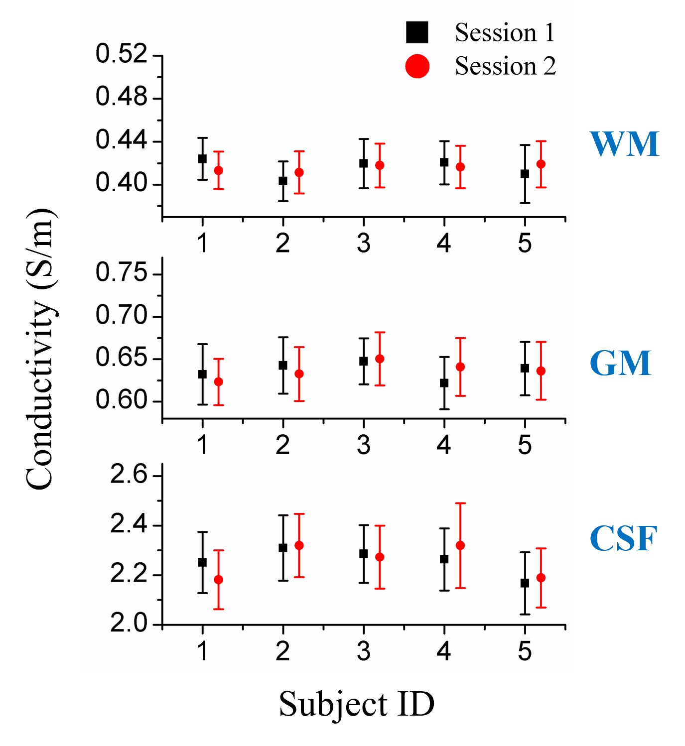
Figure 1. Conductivity
values (with error bars) of five healthy subjects undergoing scans on two
separate days. The measured mean and variance of conductivity values of
white matter, gray matter and CSF at 3T Larmor frequency were 0.42 ±
0.02,
0.63 ±
0.03,
2.24 ±
0.10
S/m.
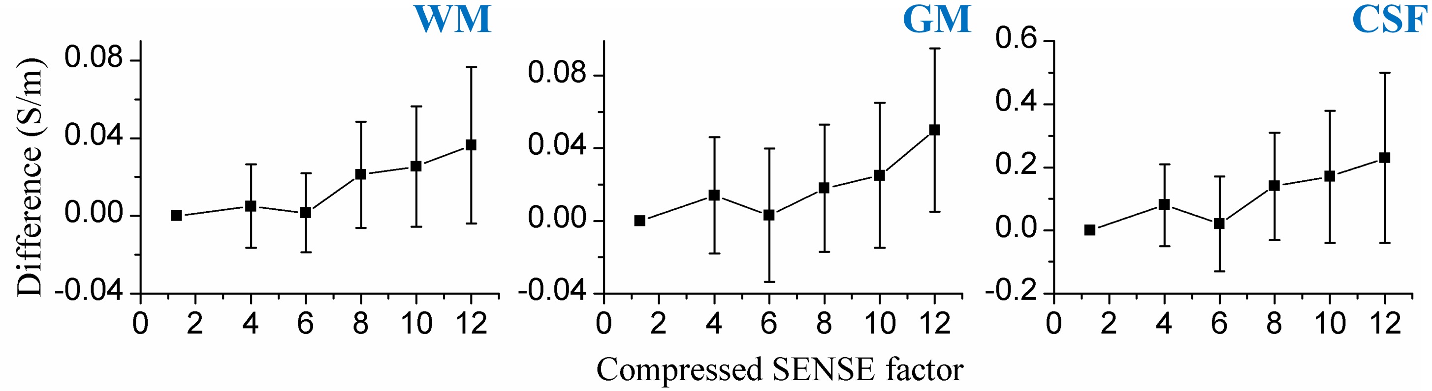
Figure 2. Conductivity variance of white matter, gray
matter and CSF with increasing CS factors. Conductivity difference was
made by subtracting the conductivity maps with higher CS factors (from 2 to 12) from the reference conductivity map (CS factor 1.3). The conductivity of
white matter had minimal deviation with CS factor up to 5 with deviations increasing
at CS factors > 6. The conductivity of gray matter had minimal deviation up
to CS factor 6 with increasing deviation at CS factor >8.
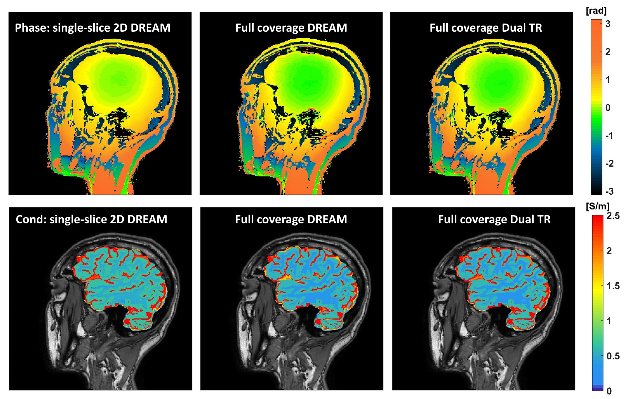
Figure 3. Phase and conductivity maps of one sagittal
slice of the same healthy subject scanned with BFFE using single-slice 2D DREAM, BFFE using full
coverage DREAM and BFFE using full coverage dual TR approach, respectively.
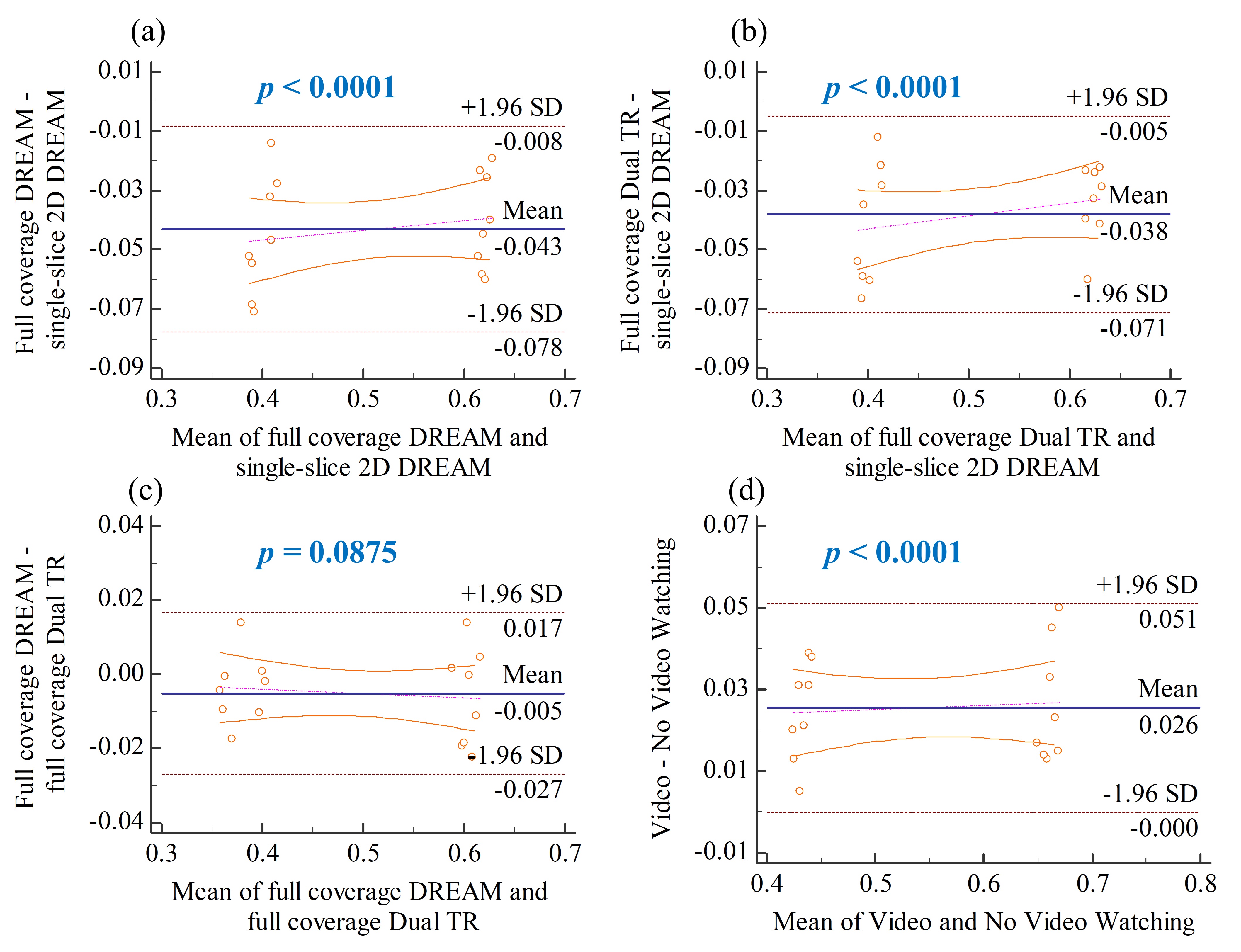
Figure 4. Bland-Altman plots of conductivity measurements
and p-values of paired t-test (α = 0.05). (a)
BFFE using single-slice 2D DREAM and BFFE using full coverage DREAM; (b) BFFE
using single-slice 2D DREAM and BFFE using full coverage dual TR approach; (c)
BFFE using full coverage DREAM and BFFE using full coverage dual TR approach;
and (d) BFFE using single-slice 2D DREAM without video watching and BFFE using
single-slice 2D DREAM with video watching.
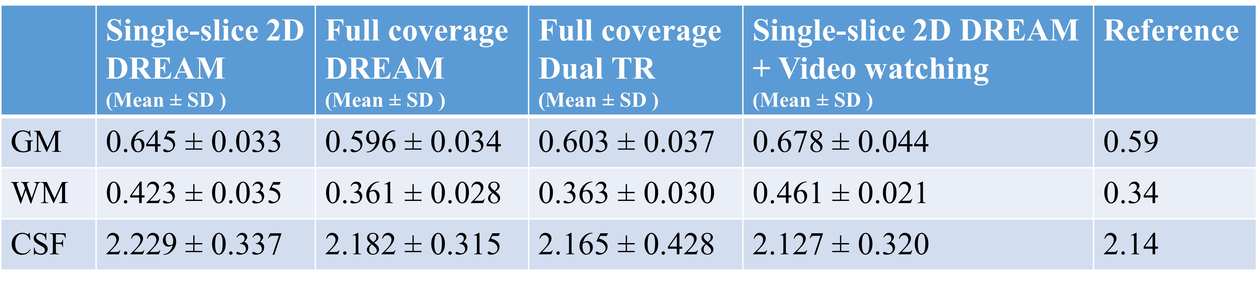
Table 1. The
conductivity measurements of one healthy subject using BFFE with three B1 mapping methods and video watching. [unit: S/m]
DOI: https://doi.org/10.58530/2022/3633