3574
Restoration of corrupted 13C MR spectroscopy with signal overflow
Leon Sergey Khalyavin1 and Jae Mo Park1
1University of Texas at Dallas, Richardson, TX, United States
1University of Texas at Dallas, Richardson, TX, United States
Synopsis
This study aims to reconstruct 13C spectrum from FID that is corrupted by signal overflow. As the corruption often occurs in the beginning of the FID, an uncorrupted section can be reconstructed as a time-delayed version of the FID. The T2*, M0, and frequency of metabolite peaks can be calculated from the reconstructed spectrum of the uncorrupted FID signal. Since the T2* is an innate property of the compound, it can be used to extrapolate the M0 of the original signal using a mono-exponential function for each peak. The method was tested with dynamic hyperpolarized 13C MRS data.
Background
Free induction decay (FID) signals can be corrupted due to various potential reasons such as additive noise from hardware or signal overflow. In particular, signal overflow is not uncommon for 13C MR data, acquired with an injection of hyperpolarized (HP) substrate, primarily due to its large signal amplification (>10,000´) and the absence of 13C signals for pre-scans, possibly resulting in the mis-calibrated receive gains. With the expenses and efforts of running such a complicated scan, it is frustrating to discard the corrupted HP data with signal overflow. This study presents a method that restores partially corrupted FID signals by fitting the key parameters such as T2*, M0, and resonance frequency of each metabolite peak from the uncorrupted FID region.Methods and Theory
An FID signal consists of 4 major components: signal intensity (M0), T2*, frequency, and phase shift. An FID signal that includes finite number (n) of frequency components can be described by eq 1. $$x(t)=\sum_n M_{n}*e^{j2\pi*f_{n}*t}*e^{-\frac{t}{T_{2,n}^{*}}}\Leftrightarrow X(f)=\sum_n \frac{M_{n}*T_{2,n}^{*}}{1+[2\pi*T_{2,n}^{*}*(f-f_{n})]^{2}}*(1+j2\pi*(f-f_{n}*T_{2,n}^{*})$$(eq. 1)As the amplitude of each peak in the spectrum is M0×T2* and the area of the peak is M0, T2* can be calculated from the full width half maximum (FWHM). By delaying the FID in time to exclude the corrupted region (e.g., t0), an additional linear phase term is introduced, as described in eq 2. $$x(t-t_{o})\Leftrightarrow X(f) = e^{-j2\pi*t_{o}f}*\sum_n\frac{M_{n}*T_{2,n}^{*}}{1+[2\pi*T_{2,n}^{*}*(f-f_{n})]^{2}}*(1+j2\pi(f-f_{n})*T_{2,n}^{*})$$(eq. 2)
Using the calculated T2* and unchanged resonance frequency of each metabolite peak, the M0 can be estimated by advancing the FID, extrapolating the mono exponential decay (exp(-t/T2*)).
A time-resolved cardiac 13C MRS data that was acquired from a healthy subject after a bolus injection of hyperpolarized [1-13C]pyruvate was used to test the restoration method. The data was collected using a 3T wide-bore MR scanner (750w, GE Healthcare), a SPINlabTM polarizer (GE Healthcare), and a dual-loop Helmholtz 13C TR coil (PulseTeq) were used. Other experimental details are identical to the previous study (1). The restoration accuracy of the method was validated by monitoring T2* and M0 from an uncorrupted FID with incremental delays. Finally, a corrupted FID was restored using the method.
All processing and analysis were performed using MATLAB, laid out in the flowchart, Figure 1. Briefly, the FID signal was taken with a certain amount of delay. Figure 2 shows the FID signal and spectrum. M0, T2*, M0T2*, and fn were calculated using the spectrum magnitude. Using T2*, the values were then extrapolated to find the uncorrupted values. Using eq. 2, the peaks were then reconstructed and summed together to create the new spectrum.
Results and Discussion
With increase delay, the reconstructed M0 and T2* should be constant. As seen in Figure 3, M0 tends to be relatively constant until delay 2000. At that moment, the SNR is too large and therefore, it is difficult for the computer to calculate the values for T2* and M0. It is highly likely a user would reconstruct a spectrum at that delay, therefore it is not an issue. At high SNR, the performance of the algorithm decreases. This might be able to be fixed by applying a filter onto the spectrum.The T2* values are relatively constant as well. There is a slight decrease as the delay increases. This is because the body circulates the groups out, which leads the T2* to be imprecise. This leads to a slight decrease in the estimated M0, which can be seen on the graph. The decrease is relatively small and is linear with respect to delay. This was later fixed by adding a linear component that increases with respect to delay for each peak. This linear component would increase with more delay, which would counteract the decrease in T2*. This significantly improves the performance of the algorithm at higher delays, since it adjusts the T2* values to where they should be.
Figure 4 shows the performance of the algorithm under different delays. The first graph shows the spectra with 0 delay. Theoretically, the reconstructed signal should map identically onto the original signal, which it does. The peaks are similar height, with the height difference accounted for by the rolling base on the original spectrum. The second graph shows 200 delay. The graph shows a good increase in the peak values. The third graph shows the comparison of the two reconstructed graphs. The frequency and the width of the graphs line up almost perfectly, while there is some variation with the peak heights. This is due to the inconsistency of calculating the T2*, most likely due to the groups leaving. With higher delay, the more inconsistent the graphs will become.
This algorithm is intended to restore corrupted data. Figure 5 shows a corrupted signal, with the highlighted portion showing the corrupted section. The second graph shows that the spectrum is barely readable. A delay was taken of 300, when the signal was not corrupted, and the spectrum was restored. As shows, the spectrum was able to be restored with similar peak heights to the uncorrupted spectra. This verifies the performance of the algorithm.
Conclusion
This method demonstrates that corrupted FID can be restored with peak quantitation accuracy. The proposed method can be expanded to free induction decay chemical shift imaging.Acknowledgements
Funding: National Institutes of Health of the United States (R01 NS107409, P41 EB015908, S10 OD018468)References
1. Park JM, Reed GD, Liticker J, Putnam WC, Chandra A, Yaros K, et al. Effect of Doxorubicin on Myocardial Bicarbonate Production from Pyruvate Dehydrogenase in Women with Breast Cancer. Circ. Res. Lippincott Williams & Wilkins Hagerstown, MD; 2020 Oct 14;104:19773. PMCID: PMC7874930Figures
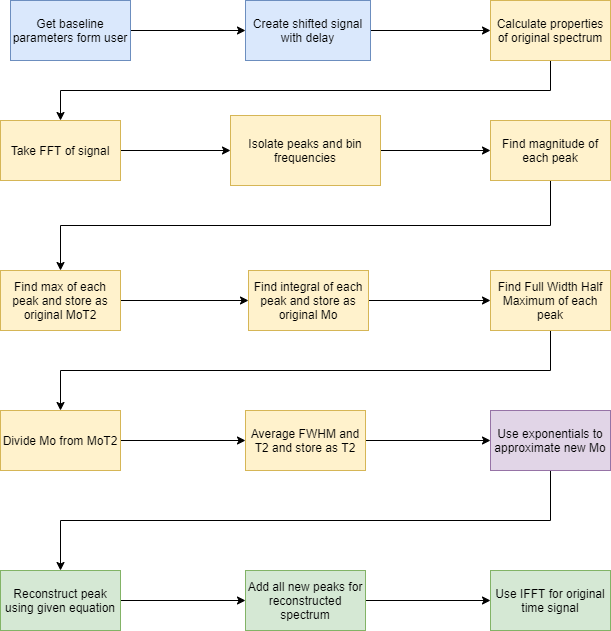
Figure 1:
Flowchart of FID reconstruction process
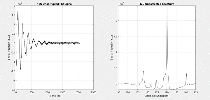
Figure 2:
Graph 13C uncorrupted signal and spectrum
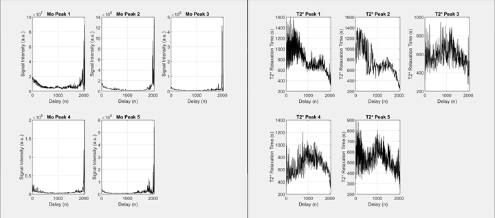
Figure 3:
Mo and T2* values and delay increases
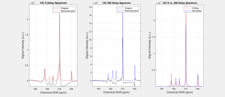
Figure 4: Spectrum reconstruction with different delays. Left and middle graph - reconstruction with delay. Right graph - comparison of graph reconstruction
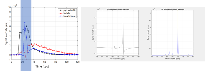
Figure 5: Restoration of corrupted FID signal. Left graph
- highlighted is corrupted area. Middle graph - corrupted spectrum. Last graph - restored spectrum.
DOI: https://doi.org/10.58530/2022/3574