3522
Efficient Network for Diffusion-Weighted Image Interpolation and Accelerated Shell Sampling1The Florey Institute of Neuroscience, Melbourne, Australia, 2MR Research Collaborations, Siemens Healthcare Pty Ltd, Bayswater, Australia, 3MR Research Collaborations, Siemens Healthcare Pty Ltd, Brisbane, Australia, 4MR Applications Predevelopment, Siemens Healthcare GmbH, Erlangen, Germany
Synopsis
We propose an efficient, densely connected network to synthesize unacquired DW-volumes from other acquired DW-directions and b=0 mm2/s volumes, allowing acceleration of high-angular DWI shell acquisition by skipping some DW-directions altogether.
For training, we used a high-quality dataset of 20 HCP subjects with 90 DW-directions per subject at both b=1000 mm2/s and 3000 mm2/s. 40 HCP subjects were used for validation. 30 DW-directions were selected for input to reconstruct the other 60 missing target DW-directions.
Comparison with a linear-interpolation benchmark show improved fidelity of synthesized DW-volumes and FOD maps to a gold standard acquisition, for both b-values.
INTRODUCTION
Fibre-tracking and fixel-based analyses are valuable tools in the study and diagnosis of neurological disorders1,2, but their adoption in the clinical practice can be hampered by long acquisition times, as they require many Diffusion-Weighted (DW) Images, typically over 60 directions and multiple b-values. Even with acceleration techniques such as simultaneous multi-slice sequences, acquisition times can be on the order of 10 minutes or more3. However, further acceleration could be achieved by skipping the acquisition of some DW directions and synthesizing missing images offline4,5.This image synthesis problem is akin to interpolation along the diffusion encoding direction in q-space4. While it is possible to perform a linear interpolation on a voxel basis5, deep-learning interpolating networks could potentially capture a more accurate diffusion model than a strictly linear one. The difficulty resides in developing a network that can extract the inherent diffusion model from training data without introducing fitting bias. Conventional Deep-Learning approaches often use a large convolution network6,7 with stringent regularization on the trained parameters, on a very large training set. We demonstrate here that a relatively shallow but densely connected network can instead be used, even with a relatively small number of training subjects, with clear improvement over a linear interpolation model.
METHODS
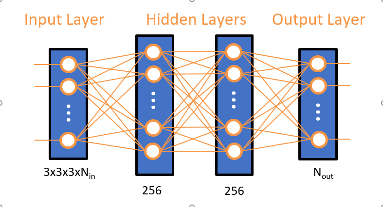
Network development was performed using TensorFlow8. The proposed network is shown in figure 1. It synthesizes each of the Nout target DW-volumes on a per-voxel basis from Nin acquired DW and b=0 s/mm² volumes. The acceleration factor R for a given shell acquisition is therefore R= Nin / (Nin+ Nout).The input layer takes Nin blocks of size 3x3x3 centred around the target voxel location, followed by 2 dense layers of 256 neurons each, and an output layer producing Nout voxels. Each layer uses a “reLU” activation function.
Training and validation datasets were gathered from 20 and 40 subjects respectively of the Human Connectome Project database9, treated as 3D volumes of dimension 145 x 174 x 145 at 1.25mm isotropic resolution, with 90 directions at b=1000 s/mm² and b=3000 s/mm², and a single b=0 s/mm² image. The brain-masks provided by the HCP dataset were used to exclude non-brain-tissue voxels from training and validation.
The network was trained for each b-value with Nin = 31 and Nout= 60, (R≈3) . Input DW-directions were chosen to best match a 3D golden angle sampling scheme. Training using a mean-square-error loss-function was completed over 100 epochs on the MASSIVE supercomputer10 using 192 GB of RAM.
As a benchmark comparison, a linear interpolation model was also trained from the same datasets.
For each model and each b-value shell, Fibre Orientation Distribution (FOD) maps were computed from the input and synthesized volumes, using Constrained Spherical Deconvolution (CSD)11 with MrTrix312, and compared with FOD maps from fully sampled shells.
RESULTS
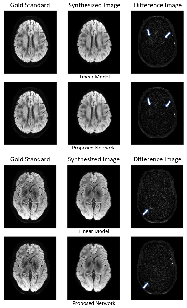
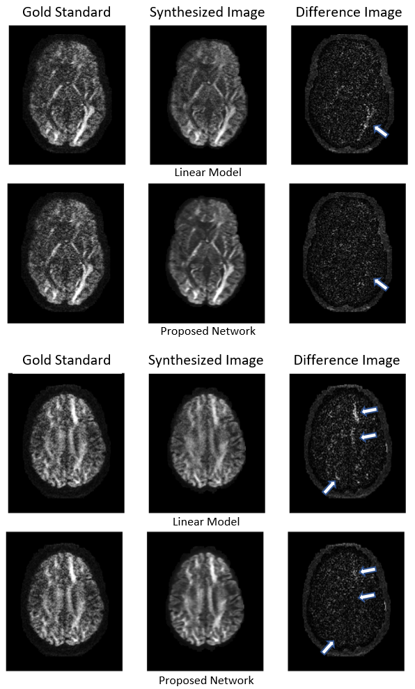
An example comparison of synthesized images for the different methods is shown in figure 2 at b=1000 s/mm² and figure 3 at b=3000 s/mm². The target image as acquired by the scanner is referred to as gold standard.With all models and both shells, the synthesized image appears to have a higher SNR than the gold standard, resulting in similar salt and pepper patterns in the difference image. However, the linear model exhibits local errors in regions corresponding to important fibre tracks such as the optic and thalamic radiations. In comparison, the network reconstruction showed noticeable reductions of these errors, particularly for b=3000 s/mm².
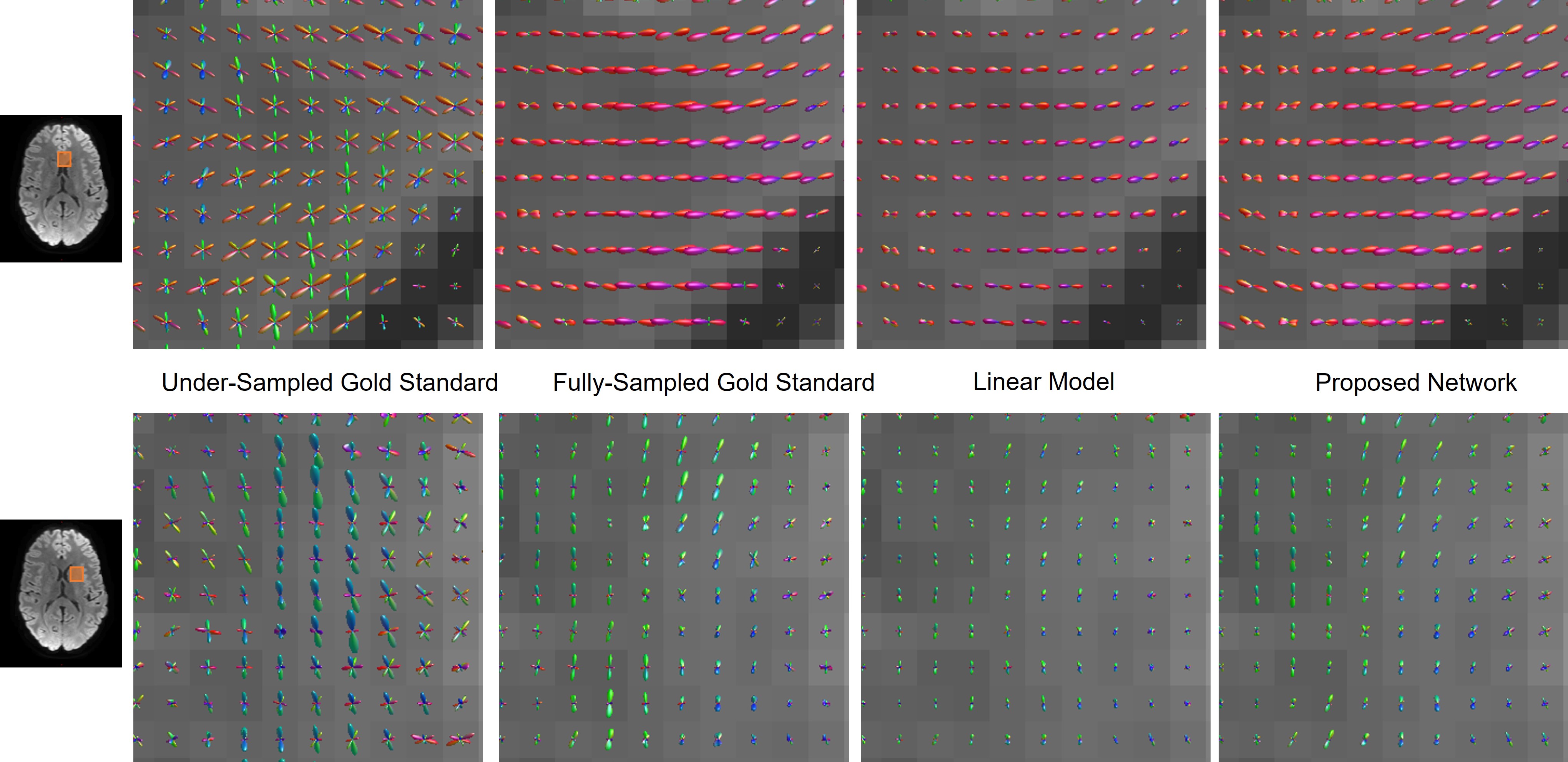
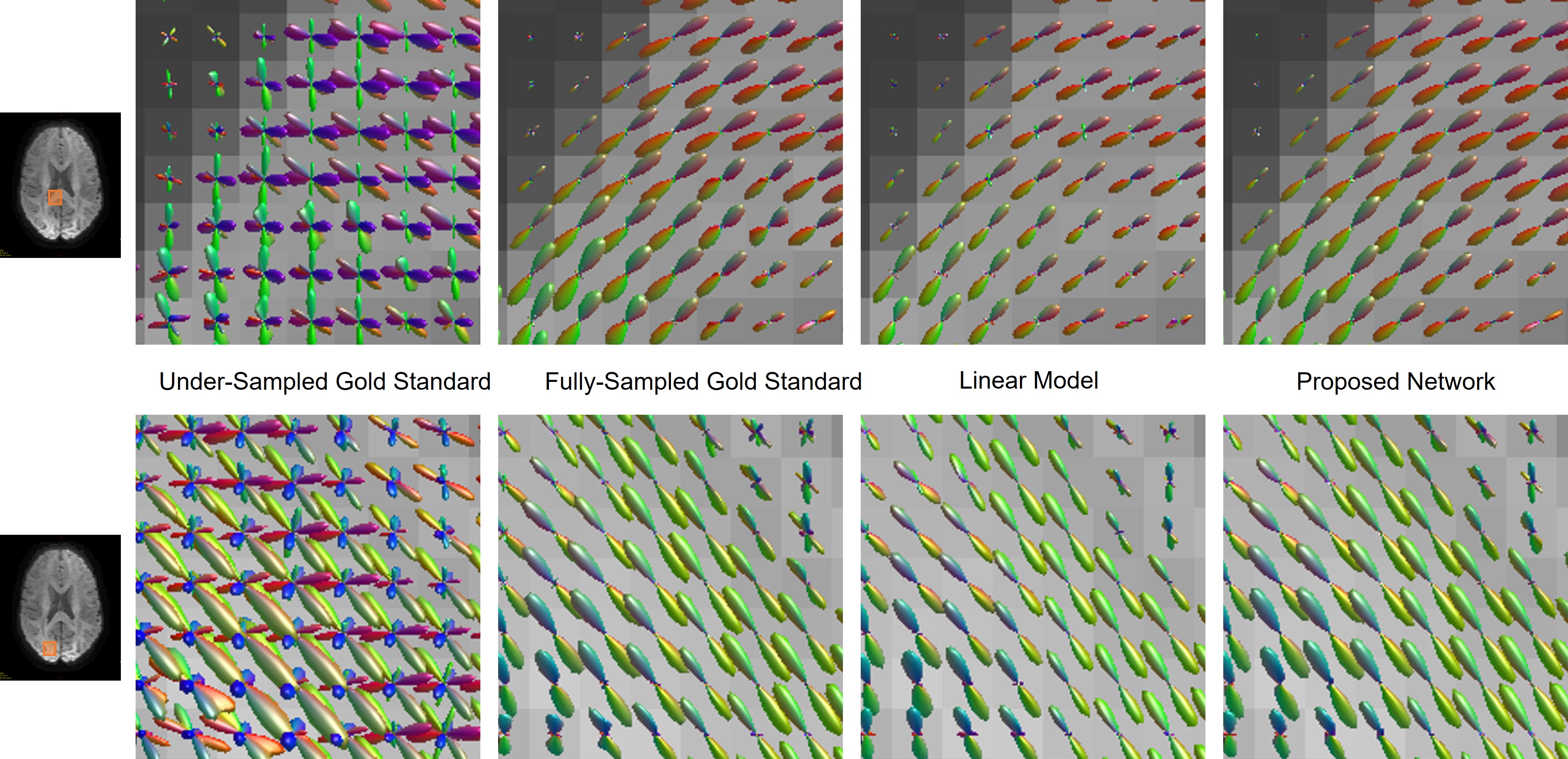
An example comparison of FOD maps is shown in figure 4 and figure 5. Using only 30 gold standard directions leads to clear errors, illustrating a need for interpolation across DW-directions. With all models, the directions of the FODs correlate with the fully-sampled gold standard, but their amplitudes often appeared slightly decreased with the linear model. FODs reconstructed with the deep-learning network do not exhibit such an amplitude reduction.
DISCUSSION & CONCLUSION
The proposed network is small but highly non-linear and enables the use of spatial-neighbourhood information. It appears to capture a better inherent diffusion model than the linear interpolation approach, particularly for higher b-values. One benefit of the small number of parameters is fast, reproducible training without need for additional regularization. It should be noted that deeper networks (up to 5 hidden layers), 3D convolution layers, batch normalization and weight regularization were also tested but did not yield any improvements over the presented results.The analysis of the model’s performance was somewhat limited by the SNR of the gold standard target images. The strong salt and pepper noise present in the acquired image seemed drastically reduced in the synthesized images. This leads to a discrepancy in SNR between acquired and synthesized DW-directions. The effect of SNR mismatch on FOD analysis remains to be investigated.
The training dataset was also comprised solely of healthy controls, and the viability of the network for synthesizing pathological data will also need to be investigated. However, the proposed network is a promising approach for significantly accelerating data acquisition for connectome and fixel-based analysis, with shown results corresponding to a threefold reduction in acquisition time. Furthermore, it is compatible with other acceleration techniques such as optimized shell sampling and multi-band acceleration.
Acknowledgements
The authors would like to thank NeuroScience Victoria for support, and prof. Graeme Jackson, Dr Robert Smith and Dr Boris Mailhe for valuable input.References
1. Dhollander T, Clemente A, Singh M, et al. Fixel-based Analysis of Diffusion MRI: Methods, Applications, Challenges and Opportunities. Neuroimage. 2021;241:118417
2. Fornito A, Zalesky A, Breakspear M. The connectomics of brain disorders. Nat Rev Neurosci. 2015;16:159–172
3. Tong Q, He H, Gong T, et al. Multicenter dataset of multi-shell diffusion MRI in healthy traveling adults with identical settings. Sci Data. 2020; 7:157
4. Tuch DS. Q-ball imaging. Magn Reson Med 2004; 52:1358–1372
5. Descoteaux M, Angelino E, Fitzgibbons S, et al. Regularized, fast, and robust analytical Q-ball imaging. Magn. Reson. Med. 2007;58:497–510
6. Upchurch P, Gardner J, Pleiss G et al. Deep Feature Interpolation for Image Content Changes. 2017 IEEE Conference on Computer Vision and Pattern Recognition (CVPR), 2017, pp. 6090-609
7. Hung KW, Wang K, Jiang J. Image interpolation using convolutional neural networks with deep recursive residual learning. Multimed Tools Appl. 2019; 78:22813–22831
8. Abadi M, Agarwal A, Paul Barham P, et al. TensorFlow: Large-scale machine learning on heterogeneous systems, 2015. Software available from tensorflow.org.
9. Rosen B, Toga AW, Weeden VJ. The Human Connectome Project (HCP) database. https://ida.loni.usc.edu/login.jsp.
10. Goscinski WJ, McIntosh P, Felzmann UC, et al. The Multi-modal Australian ScienceS Imaging and Visualisation Environment (MASSIVE) high performance computing infrastructure:applications in neuroscience and neuroinformatics research. Front Neuroinform. 2014;8.
11. Tournier JD, Calamante F, Connelly A. Robust determination of the fibre orientation distribution in diffusion MRI: non-negativity constrained super-resolved spherical deconvolution. Neuroimage. 2007; 35:1459–72
12. Tournier JD, Smith RE, Raffelt D, et al. MRtrix3: A fast, flexible and open software framework for medical image processing and visualisation. NeuroImage. 2019; 202:116–37
Figures