Introduction

Magnetic resonance fingerprinting (MRF) [1] is a novel multi-parametric quantitative MRI approach, where quantification maps and images of multiple contrasts can be acquired in a single scan. In this study, an MRF strategy for simultaneous T₁, T₂ and T₂* quantification of human brain is proposed using dual-echo echo planar imaging (EPI) readout and validated in brain tumor patients.

Methods

Acquisition: An IR-GRE-SSFP MRF sequence is developed, shown in Figure 1. Half scan is used for the first echo for shorter echo time (TE), rendering improved T₂ weighting in its signal evolution. Each echo is from one of a 16-shot readout, and a Blip Up and Down Acquisition (BUDA)-like [2] sampling strategy is utilized. Both the shot index and phase encoding polarity are alternated between the 2 echoes, and among consecutive time frames, ensuring better k-space coverage and incoherence of image artifacts along time axis. Variable flip angle (maximum 70 degree) and constant repetition time (TR) are used. RF spoiling is added in the first 100 time frames, making the sequence a concatenation of inversion recovery gradient echo (IR-GRE) and steady-state free precession (SSFP). The flip angle train and rf phase train are shown as Figure 2.
Reconstruction: Images for each individual lobe are reconstructed with a time-resolved [3] approach. A low rank subspace reconstruction method [4,5] is used to solve:$$\mathop{\arg \min}\limits_{\alpha}\frac{1}{2}{\parallel}FSφU_k^Hα-y{\parallel}_2^2+λ∑_r{\parallel}R(α)\parallel_*\qquad(1)$$. where $$$y$$$ is the acquired data, $$$F$$$ is Fourier transform, $$$S$$$ is coil sensitivity profile which can be self-estimated from the data by temporal sharing. $$$φ$$$ is phase increment term of off resonance map times the echo time of each lobe. The off resonance map is calculated from the phase change of 2 echoes with smooth spatial variation as a priori. $$$U_k$$$ is suppressed from singular value decomposition (SVD) of pre-calculated dictionary, with the first k singular vectors as subspace bases. $$$α={U_k}x$$$ is the subspace representation of image series $$$x$$$. A locally low rank (LLR) term is used as regularization for better conditioning. Eq (1) is iteratively solved in reconstruction using alternating direction method of multipliers (ADMM) [6].
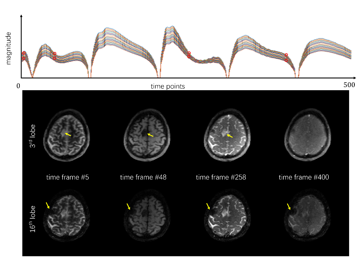
The dictionary was calculated using extended phase graph (EPG) [7] with parameters T₁ within 200~5000ms, T₂ within 20~3000ms and T₂* within 10~100ms, yielding 332672 dictionary entries of all 23 EPI lobes at 500 timeframes. A comparison of the signal evolutions of different EPI lobes was shown in Figure 3 for the dictionary entry with T₁ = 800ms, T₂ = 80ms and T₂* = 40ms. By SVD, the first 5 singular vectors were selected to ensure <0.2% error after compression, thus $$$23\times500=11500$$$ time points were represented by 5 subspace bases. Since T₁ and T₂ affect the signal evolution across different TRs, T₁ and T₂ maps as well as proton density were presented by dictionary matching. However, T₂* weighted the images within each TR, so T₂* was estimated by parameter fitting of the straightforward $$$e^{-t/T_2^*}$$$ decay term.
Experiments: All the in-vivo data were acquired on a GE 3T scanner (MR750, Waukesha, WI) with a 32-channel head coil. Other parameters included: TR = 33ms, TE1 = 4.4ms, TE2 = 20ms, FOV = 224mm², resolution = 1 mm² and EPI echo spacing = 1.2ms. 500 timeframes were acquired for each slice, and the scan time is 16s per slice. Patients with lower grade glioma were consented for evaluating the performance of the sequence. The study was approved by the Institutional Review Board.

Results

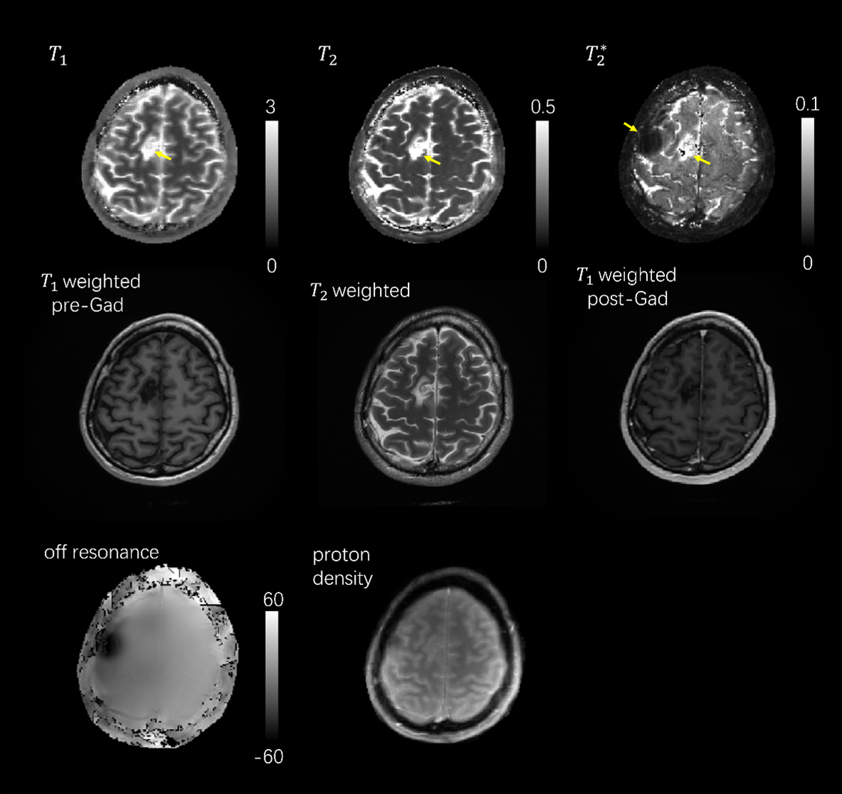
Figure 3 shows the multiple-contrast images of a grade 2, post-surgical resection, glioma patient based on the dynamic images of different time frames (namely 5th, 48th, 258th and 400th timeframes). Intensity changes due to T₂* decay was shown with the comparison of 2 readout lobes of each selected TR#. Tumor area can be observed in the images and an area with increased susceptibility due to surgery is observed in the 16th lobe.
Figure 4 shows the quantitative maps of T₁, T₂, and T₂* after dictionary matching. Tumor area is delineated in each of the 3 maps and the area with severe susceptibility is observed in the T₂* map. Results of clinical protocols of pre/post-gadolinium T₁ weighted images from an IR-GRE sequence, and T₂ weighted image from fast spin echo (FSE) sequence are also presented as references to show the consistency between MRF quantification maps and clinical images.

Discussion

In this study, the T₂* weighting, better k-space sampling coverage and off resonance estimation from the two echoes contribute to subsequent reconstruction and parametric mapping. However, one dynamic image is reconstructed at every EPI lobe along the readout, providing more image contrasts and more accurate parameter mapping. Multiple quantitative maps including T₁, T₂, T₂*, proton density, off resonance and multiple contrast images are acquired in a single scan. The various contrasts from this method are consistent with typical clinical scans. Off resonance and proton density maps from MRF reconstruction have shown potential to provide additional information. Further implementation would be improving the efficiency of the acquisition by using fewer time frames and 3D acceleration.

Conclusion

This application of MRF has demonstrated the potential to obtain quantitative relaxation maps of the brain simultaneously, saving valuable clinical scan time.

Acknowledgements

No acknowledgement found.