3494
MRI contrast synthesis from low-rank coefficient images
Xiaoxia Zhang1, Sebastian Flassbeck1, and Jakob Assländer1
1Center for Biomedical Imaging, Department of Radiology, New York University Grossman School of Medicine, New York University, New York, NY, United States
1Center for Biomedical Imaging, Department of Radiology, New York University Grossman School of Medicine, New York University, New York, NY, United States
Synopsis
Synthetic contrasts are commonly derived from parameter maps via Bloch simulation.Typically, model imperfections, in particular partial volume effects, cause artifacts in those images. Recently, it has been proposed to overcome this problem by mapping directly from MR-Fingerprinting data to synthetic contrasts with neural networks. Those methods, however, face the MRF-typical undersampling artifacts, as well as the computational burden of hundreds of input images. We propose to first reconstruct images in a low-rank sub-space, which maintains the correct partial volume contrast, but allows for removal of undersampling artifacts, and to map from this space to synthetic contrasts with a neural network.
Introduction
MR contrast synthesis from parameter maps is a catalyst for bringing quantitative MRI to the clinical practice, as it potentially allows to replace clinical scans with quantitative ones and, thus, to keep the overall protocol duration within limits. Although contrast images can be synthesized from quantitative maps, e.g., with Bloch simulations[5], those simulations commonly cause artifacts due to model imperfections, in particular at the interface between different tissues where the signal is a super-position of different contributions[10, 5, 8]. Recent deep learning methods overcome this issue by synthesizing contrasts directly from the raw data of the quantitative scan, in particular from MR Fingerprinting data[ 6, 11, 12, 13]. However, typical MRF data is highly undersampled, which causes severe artifacts when using the typical back-projection reconstruction. Thus, extra measures have to be taken to account for those artifacts, in particular, for the non-Gaussian statistics of the artifacts[11].Here, we propose to overcome these limitations by first reconstructing images into a low-rank subspace[7, 9, 2]. Such a reconstruction allows for the removal of undersampling artifacts and, due to the linearity of the reconstruction, it maintains the super-position of different signals.
Methods
Data acquisition and preprocessing: On a 3T scanner and after getting informed consent, we scanned 6 subjects (3 asymptomatic volunteers, 2 multiple sclerosis, and one brain tumor patient, where the first 5 serve as training and the last as a test dataset). We acquired MP-RAGE images andMRF-like datasets with a magnetization transfer (MT) hybrid-state pulse sequence.[3, 1] Both scans image the whole brain with an isotropic resolutions of 1mm3, and we note that this qMT sequence encodes all major mechanisms that contribute to the MP-RAGE contrast.We calculated 13 basis functions by taking an SVD of a dictionary that contains simulated signals,[7]and reconstructed coefficient images directly in this low-rank sub-space,[9, 2] which removes virtually all undersampling artifacts (Fig. 3).As sketched in Fig. 2, we feed the 13 coefficients of each voxel in a 5×5×5 cube, i.e., 13x125data-points, into a neural network to synthesize an MP-RAGE contrast in the central voxel. All input data-points, as well as the ground truth MP-RAGE signal were normalized by the complex-valued first coefficient of the central voxel. As the spin evolution in the hybrid state stays on one axis in the complex plane, we discard the imaginary part after the normalization. The final contrast value is given by the product of the network estimate and the normalization factor. This normalization minimizes the data variability that is caused by coil sensitivities etc.
Network Structure: The fully-connected network is composed of an input layer followed by eight hidden layers and an output layer. This network was defined in the pytorch-framework and is depicted in Fig. 2. All hidden layers are followed by batch normalization and rectifier linear unit (ReLU)activation functions. An L2 loss is used for training.
Synthesis via Bloch-McConnell Simulation: For comparison, we also calculate synthetic contrast with explicit Bloch-McConnell simulations from the quantitative magnetization transfer(qMT) parameter maps. After the inversion, we model the coupled recovery with a Bloch-McConnell equation[4] and simulate the turbo-FLASH readout with Bloch simulations of multiple isochromats.
Results
Fig. 4 compares a clinical (ground truth) and synthetic MP-RAGE images in a representative training dataset. Overall, both approaches are able to generate images that resemble the MP-RAGE contrast.However, the Bloch-McConnell simulation is unable to capture partial volume effects, which results in well-known artifacts at GM-CSF interfaces. This is most pronounced around the gyri, sulci, and the cerebellum. The proposed neural network models the partial volume effects more accurately and. the depiction of the tissue interfaces closely resembles the clinical MP-RAGE. Fig. 5 depicts the test data of a brain tumor patient. While the image quality is inferior in all three contrasts, we obverse reasonable generalization of the network. We note the small number of training datasets (5) and unseen pathology.Discussion and Conclusion
We demonstrated that coefficient images of a low-rank basis provide a useful intermediate stepfor generating synthetic contrasts from MRF-like data: it allows for the removal of undersamplingartifacts (cf. Fig. 3), while it correctly describes the super-position of different signals by virtue ofthe linearity of the reconstruction. This steps provides the basis for a comparably small network toadequately estimate synthetic contrasts. Future work will include the acquisition of more trainingdata, with a focus on diverse pathologies, which should improve the generalization of the network.Further, we will explore advanced loss functions and network architectures. Last, we will trainnetworks that synthesize different contrasts, such as T2w and FLAIR from the same qMT data, as itencodes all contrast mechanisms relevant for these pulse sequences.Acknowledgements
This work was supported by grant NIH/NIBIB R21 EB027241 and NIH R01 AR076985 and was performed under the rubric of the Center for Advanced Imaging Innovation and Research, a NIBIB Biomedical Technology Resource Center (NIH P41 EB017183).References
- J. Assländer and D. K. Sodickson. Quantitative Magnetization Transfer Imaging in the HybridState. InProc. Intl. Soc. Mag. Reson. Med. 27, page 1104, 2019.
- J. Assländer, M. A. Cloos, F. Knoll, D. K. Sodickson, J. Hennig, and R. Lattanzi. Lowrank alternating direction method of multipliers reconstruction for MR fingerprinting.Magn.Reson. Med., 79(1):83–96, jan 2018.
- J. Assländer, D. S. Novikov, R. Lattanzi, D. K. Sodickson, and M. A. Cloos. Hybrid-statefree precession in nuclear magnetic resonance.Nat. Commun. Phys., 2(1):73, dec 2019..
- D. F. Gochberg and J. C. Gore. Quantitative imaging of magnetization transfer using aninversion recovery sequence.Magn. Reson. Med., 49(3):501–505, 2003. .
- A. Hagiwara, M. Warntjes, M. Hori, C. Andica, M. Nakazawa, K. K. Kumamaru, O. Abe, andS. Aoki. Symri of the brain: rapid quantification of relaxation rates and proton density, with synthetic mri, automatic brain segmentation, and myelin measurement.Investigative radiology,52(10):647, 2017.
- D. Ma, V. Gulani, N. Seiberlich, K. Liu, J. L. Sunshine, J. L. Duerk, and M. A. Gris-wold. Magnetic resonance fingerprinting.Nature, 495(7440):187–192, 2013.
- D. McGivney, D. Ma, H. Saybasili, Y. Jiang, and M. Griswold. Singular Value Decompositionfor Magnetic Resonance Fingerprinting in the Time Domain.IEEE Trans. Med. Imaging, 33(12):2311–2322, 2014.
- D. McGivney, A. Deshmane, Y. Jiang, D. Ma, and M. A. Griswold. The Partial Volume Problemin MR Fingerprinting from a Bayesian Perspective. InProc. 24th Annu. Meet. ISMRM, page435, 2016.
- J. I. Tamir, M. Uecker, W. Chen, P. Lai, M. T. Alley, S. S. Vasanawala, and M. Lustig. T2shuffling: sharp, multicontrast, volumetric fast spin-echo imaging.Magnetic resonance inmedicine, 77(1):180–195, 2017.
- L. N. Tanenbaum, A. J. Tsiouris, A. N. Johnson, T. P. Naidich, M. C. DeLano, E. R. Melhem,P. Quarterman, S. Parameswaran, A. Shankaranarayanan, M. Goyen, et al. Synthetic mri forclinical neuroimaging: results of the magnetic resonance image compilation (magic) prospective,multicenter, multireader trial.American Journal of Neuroradiology, 38(6):1103–1110, 2017.
- J. Trzasko and A. Manduca. Local versus Global Low-Rank Promotion in Dynamic MRI SeriesReconstruction.Proc Intl Soc Mag Reson Med, 24(7):4371, 2011.
- P. Virtue, J. I. Tamir, M. Doneva, S. X. Yu, and M. Lustig. Direct contrast synthesis formagnetic resonance fingerprinting. InProceedings of the 2018 ISMRM Workshop on MachineLearning, page 676, 2018.
- G. Wang, E. Gong, S. Banerjee, H. Chen, J. Pauly, and G. Zaharchuk. Oneforall: Improving thequality of multi-contrast synthesized mri using a multi-task generative model. InProceedings ofthe 27th Annual Meeting of ISMRM, 2019.
- K. Wang, M. Doneva, T. Amthor, V. C. Keil, E. Karasan, F. Tan, J. I. Tamir, S. X. Yu, andM. Lustig. High fidelity direct-contrast synthesis from magnetic resonance fingerprinting indiagnostic imaging. InProceedings of the 28th Annual Meeting of ISMRM, volume 867, 2020.
- X. Zhang, Q. Duchemin, K. Liu, S. Flassbeck, C. Gultekin, C. Fernandez-Granda, and J. Ass-länder. Cramer-Rao bound-informed training of neural networks for quantitative MRI. pageArXiV ID: 2109.10535, 2021.
Figures
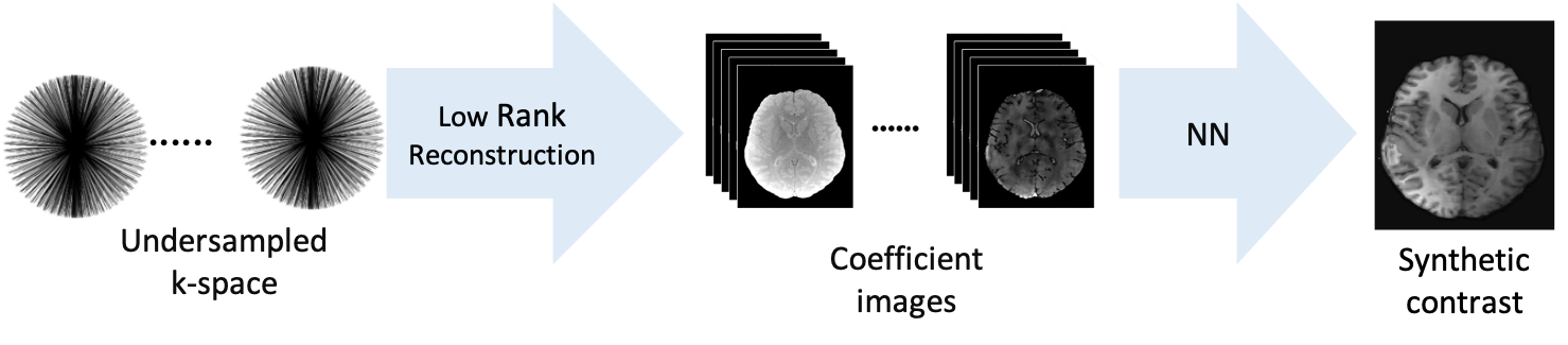
Fig. 1 Proposed pipeline to create synthetic contrasts: We first reconstruct coefficient images in a low rank space. As this reconstruction is linear, it accurately describes the super-position of signals, as common at the interface between different tissues. We then feed cubes of these coefficient images into a neural network that estimates the synthetic contrast.
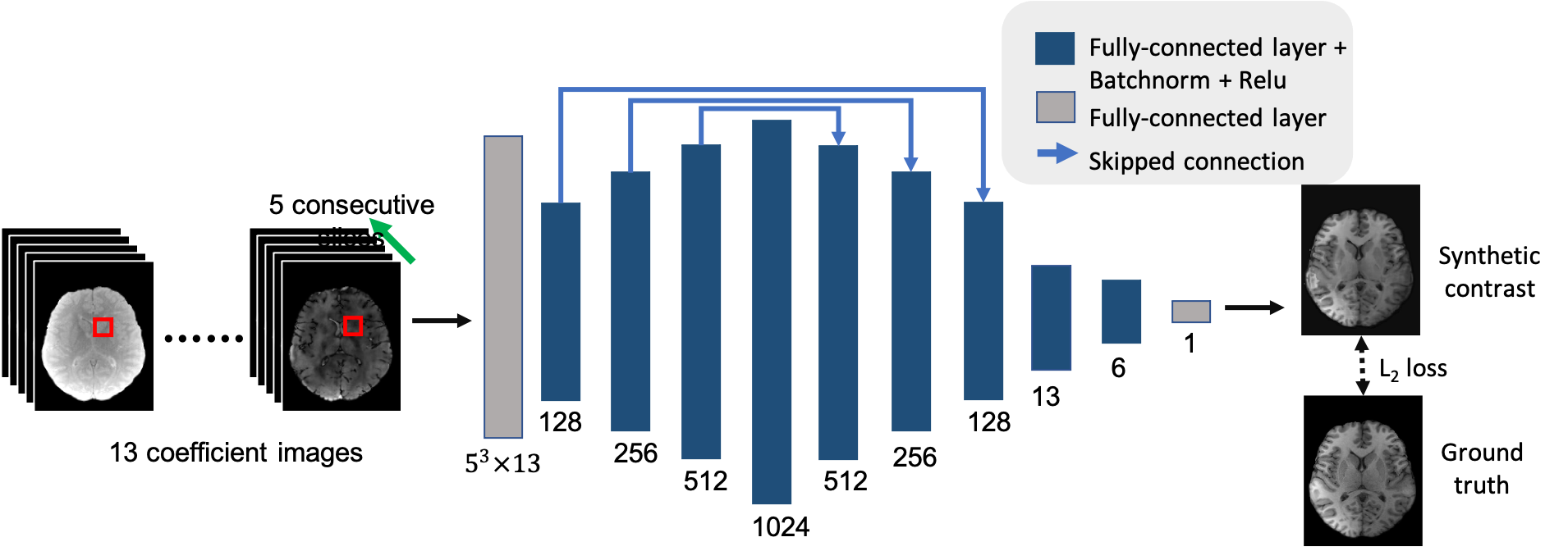
Fig. 2 Architecture of the neural network. We feed 13 coefficients of each voxel in a 5x5x5 cube, i.e., overall 13x125 data points, into the network and pass them through nine hidden, fully-connected layers, each followed by batch normalization and a rectifier linear unit activation function. The output of the network is a contrast value for the center voxel of the input 3D patch. We used an L2 loss function for training the network.
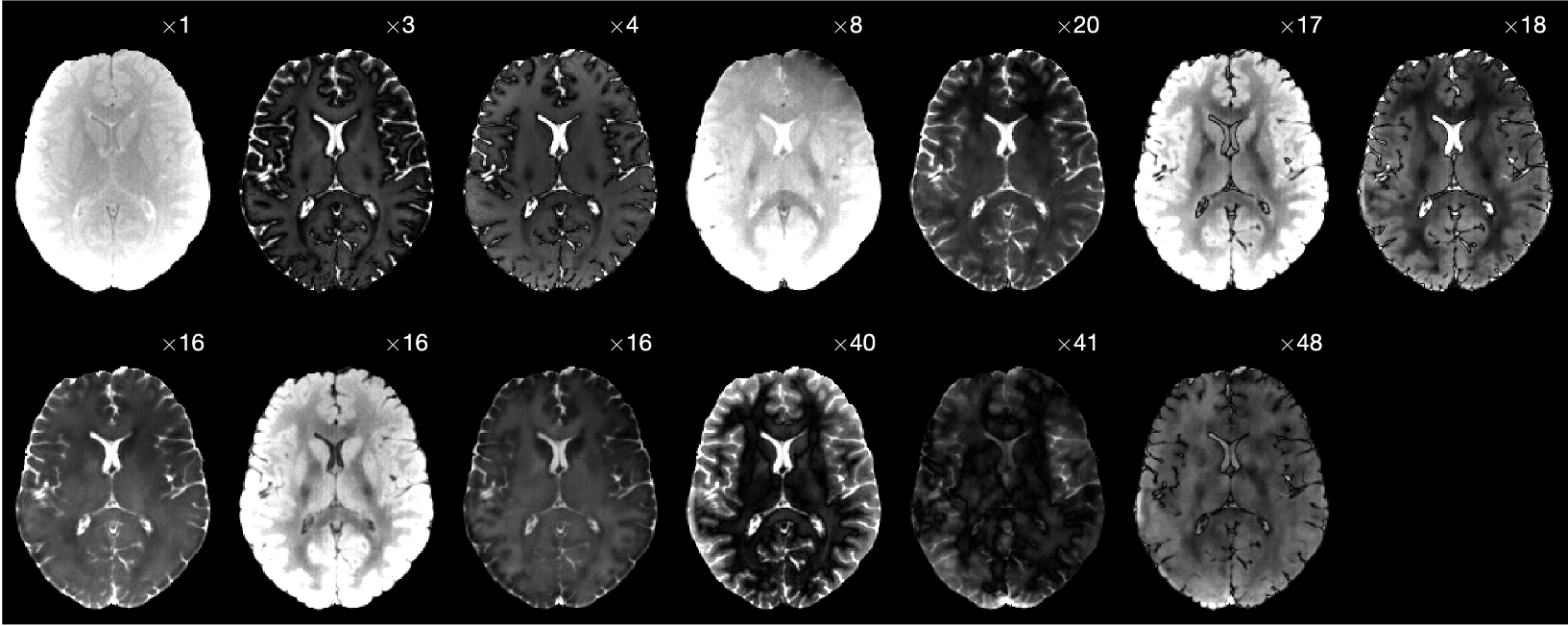
Fig. 3 A transversal slice of the 13 (3D) coefficient images that were reconstructed directly in this low-rank space. The space is spanned by the singular vectors that were calculated with an SVD of a dictionary containing simulated signals. Each coefficient image is scaled for better visualization, as indicated by the factor in the upper right corner.
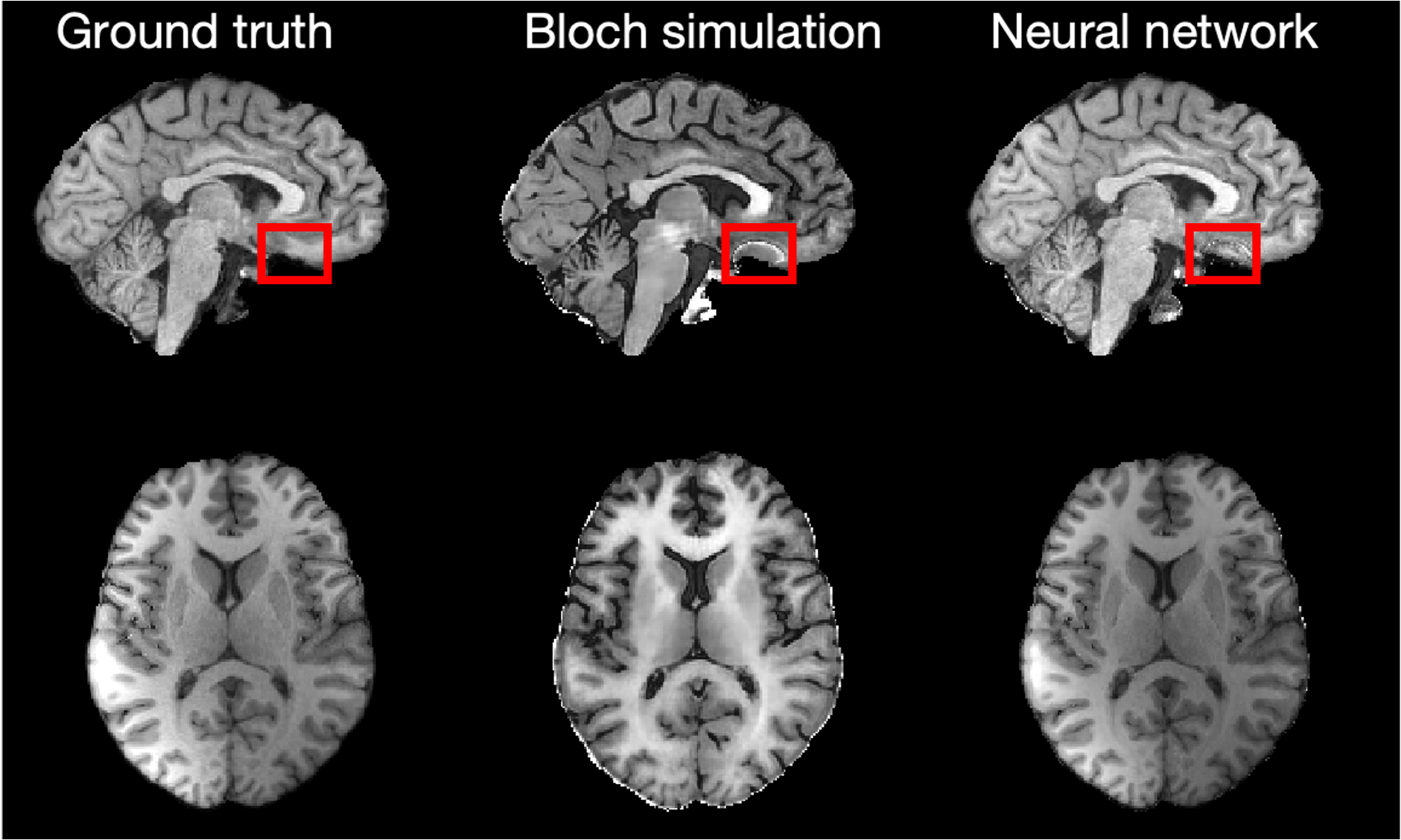
Fig. 4 Comparison of a clinical (left) and synthetic MP-RAGE contrasts that were calculated via Bloch simulations (middle) and the proposed neural network (right). When using Bloch simulations, the grey matter is thinner compared to the clinical MP-RAGE due to the partial volume effects at the GM/CSF interface. In contrast, proposed neural network network generates a synthetic contrast that resembles the clinical scan well. The red box indicated B0 banding-artefacts resulting from the balanced gradient moments in the hybrid-state qMT sequence. This was part of the training data.
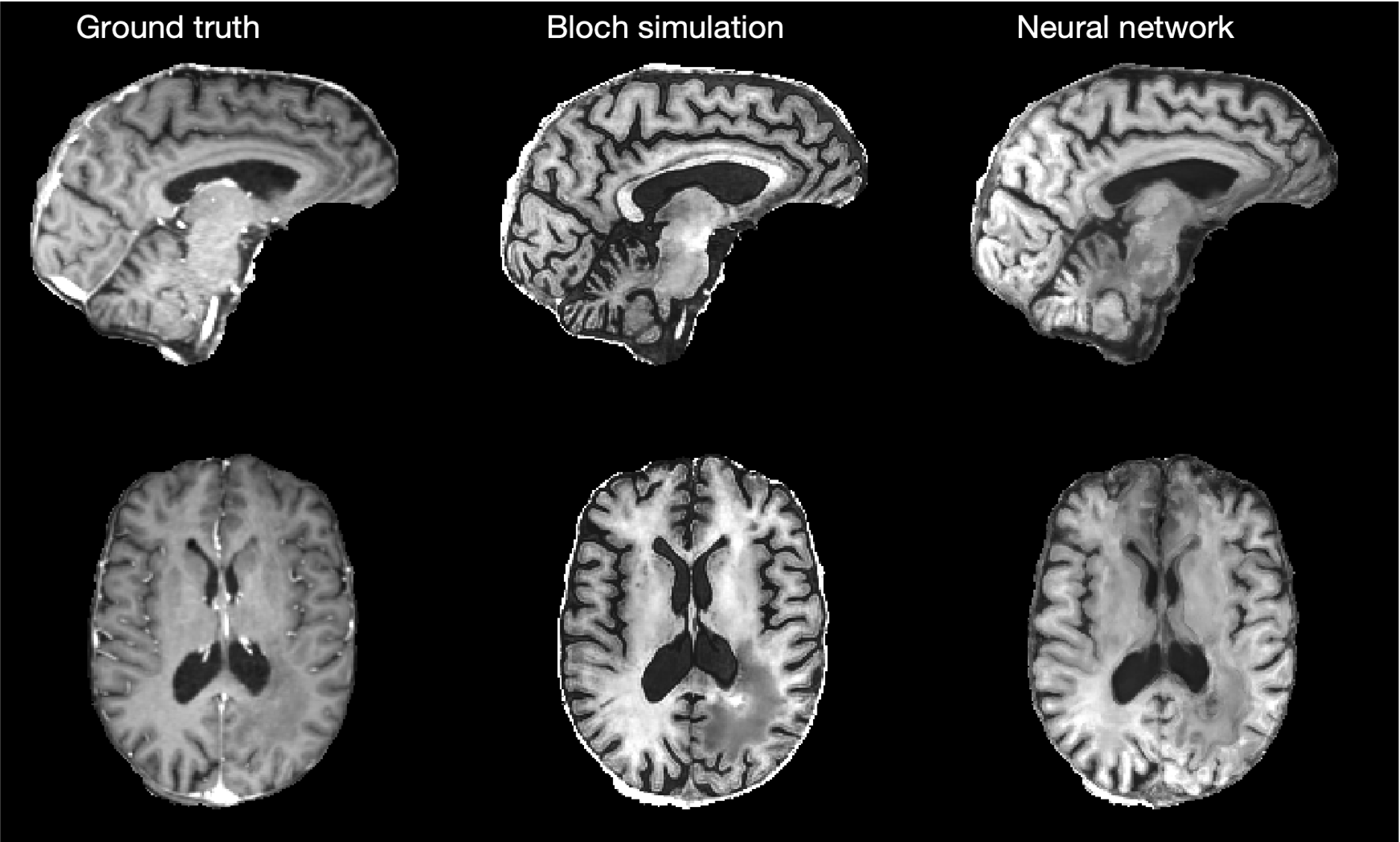
Fig. 5 Comparison of a clinical (left) and synthetic MP-RAGE contrasts that were calculated viaBloch simulations (middle) and the proposed neural network (right). This scan was not part of the training data. The image quality of all three datasets, including the ground truth, are inferior to Fig.4. Yet, it demonstrates a reasonable generalization of the network, considering the small training data set (5 scans) and the unseen pathology.
DOI: https://doi.org/10.58530/2022/3494