Introduction

Since the diffusion MRI signal can only be sampled in a finite number of directions, an experimentally estimated fiber orientation density function (fODF) is susceptible to aliasing errors. Aliasing is most familiar in the context of Fourier series representations for signals, but it is equally relevant for the spherical harmonic expansion representation of fODFs.¹ For Fourier series, oversampling at a rate higher than the Nyquist frequency is employed to suppress aliasing errors. For example, oversampling by a factor of two is conventionally used in MRI for frequency encoding of imaging data.² For spherical harmonic expansions, the analog of sampling at the Nyquist frequency is using a number of diffusion encoding directions that exactly matches the number of free parameters in the expansion. When this is done, aliasing errors are likely to occur for signals containing high angular frequencies, as is the case for fODFs with sharp peaks. Here we investigate how much oversampling is required to reduce aliasing errors. Our results may help guide the design of efficient diffusion MRI data acquisition protocols that are adequate for calculating high fidelity fODFs.

Methods

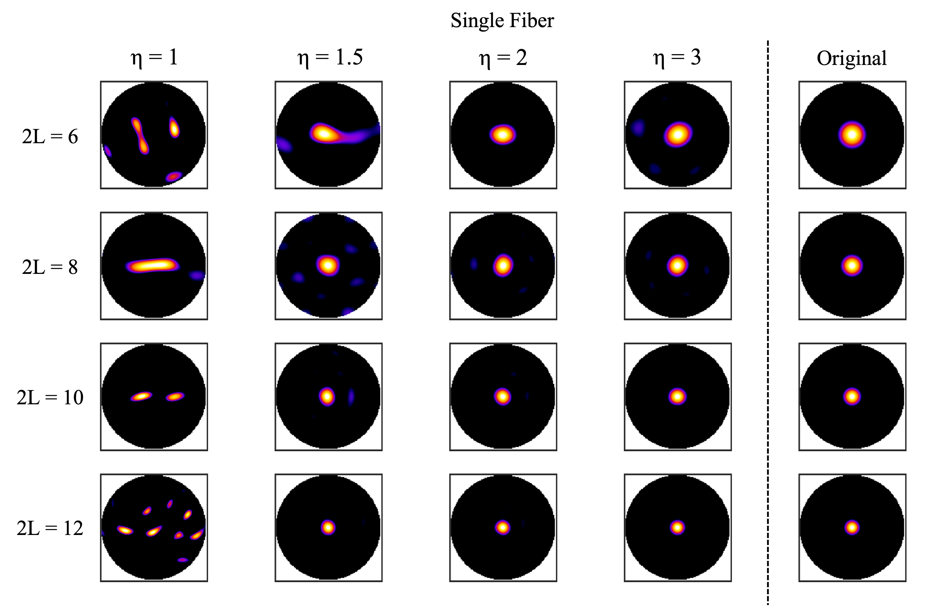
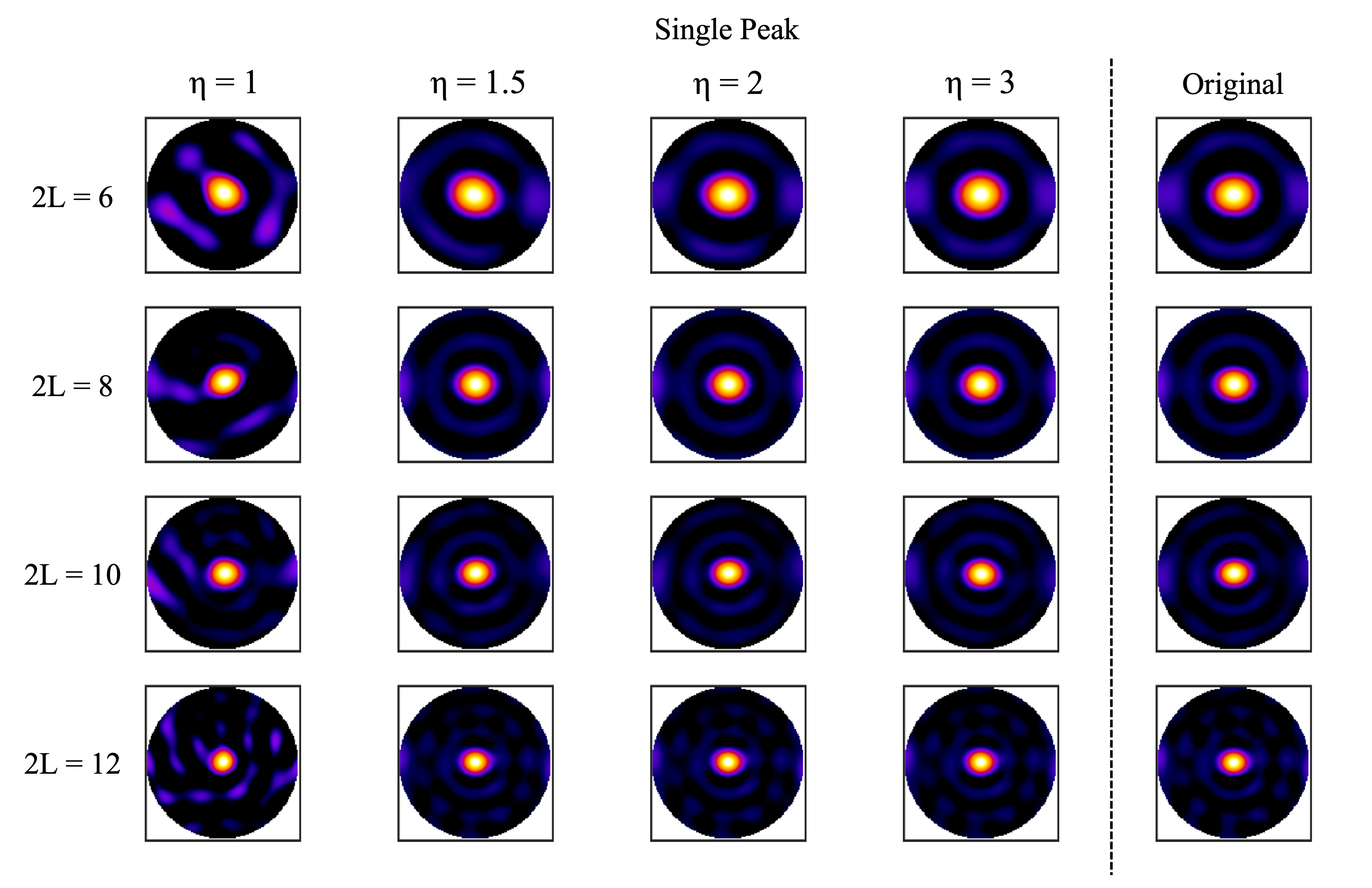
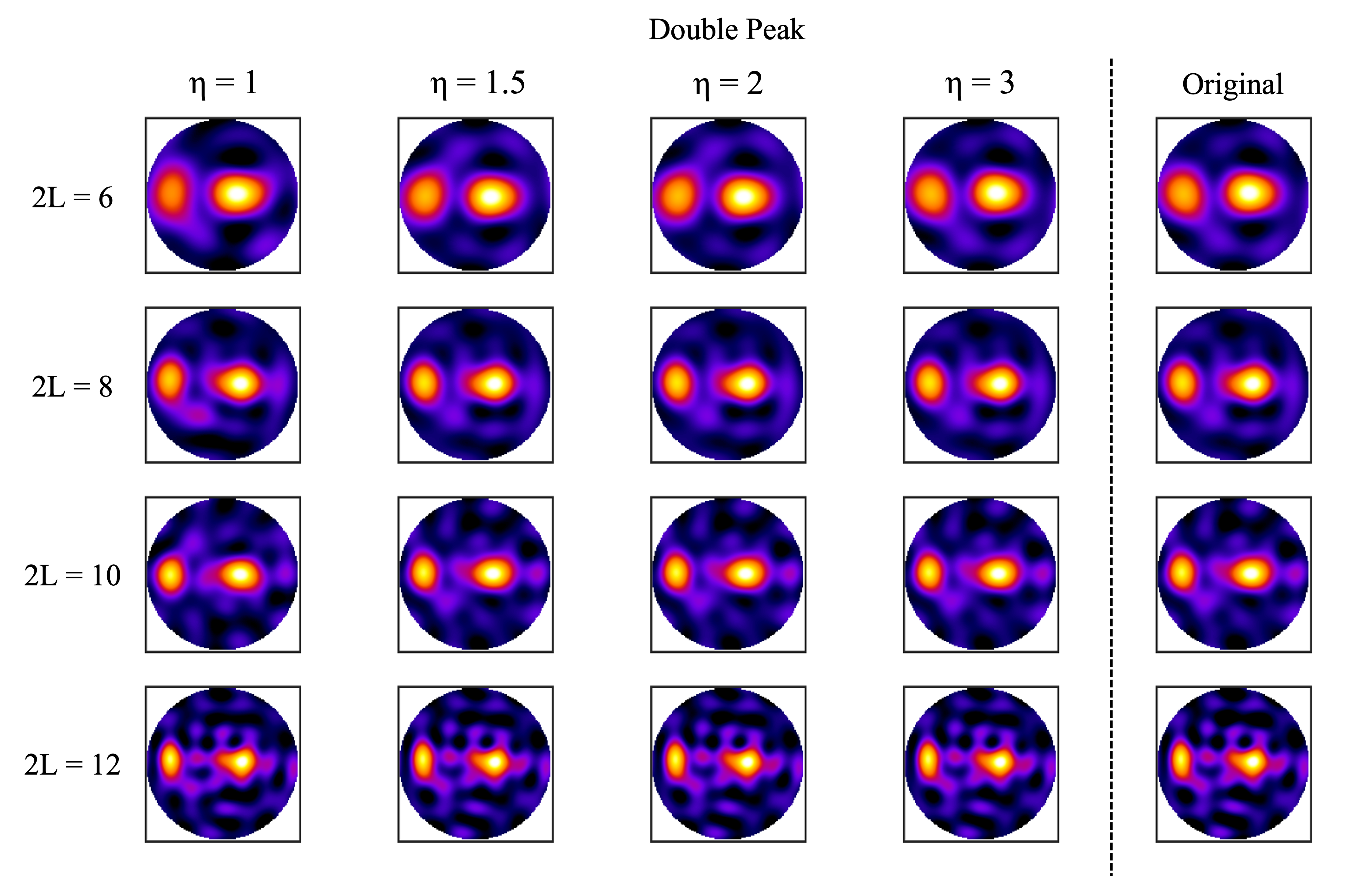
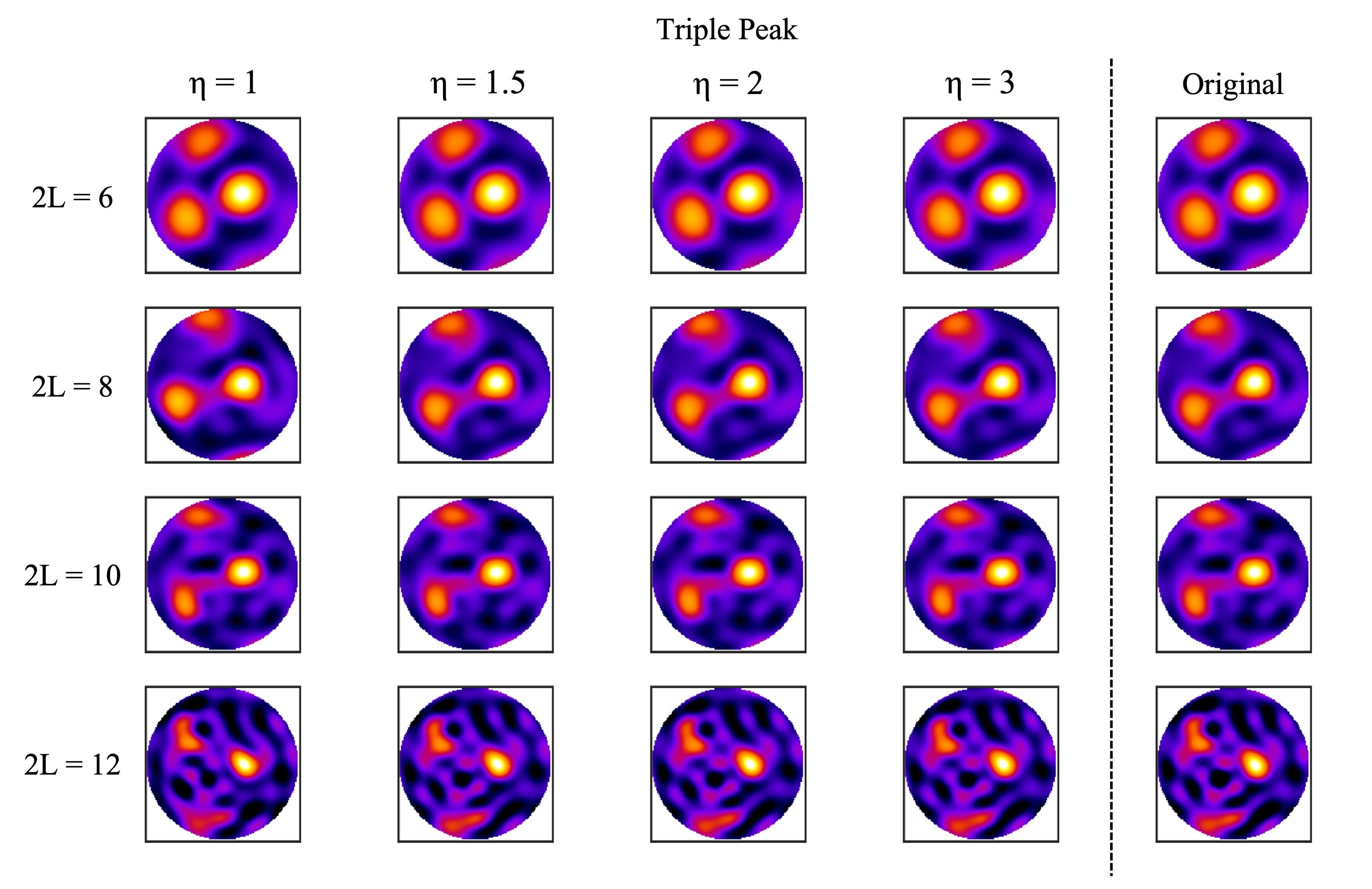
For simplicity, we assume the diffusion MRI data are acquired with a sufficiently high b-value, $$$b$$$, so signal from extra-axonal water is negligible. In practice, this means $$$b\ge 4000 \text{s/mm}^{2}$$$ for white matter in healthy adults imaged at 3T.^3,4 We also adopt the standard picture of axons being well described as thin, straight, impermeable tubes.⁵ The diffusion MRI signal, $$$S(\bf{n})$$$, is then related to the fODF, $$$F(\bf{u})$$$, by $$S({\bf n})= \frac{2 \bar{S}}{k} \sqrt{\frac{bD_{a}}{\pi}} \int d\Omega_{\bf u} F({\bf u}) \text{ exp}[-bD_{a} ({\bf n} \cdot {\bf u})^{2}] \equiv \frac{2 \bar{S}}{k} \tilde{T}_{F}\{F\}({\bf n},bD_{a}), [1] $$ where $$${\bf n}$$$ is a unit direction vector, $$$\bar{S}$$$, is the signal averaged over all directions, $$$D_{a}$$$ is the intrinsic intra-axonal diffusivity, $$$k$$$ is a normalization constant, and $$$\tilde{T}_{F}\{F\}$$$ indicates the generalized Funk transform.⁶ The integral in Equation [1] is taken over the entire unit sphere, and the normalization constant $$$k$$$ may be fixed by setting the integral of the fODF to unity. For $$$bD_{a} \gg 1$$$, we have $$$k \approx 1$$$. Equation [1] allows the exact signal function to be determined for any given fODF. Here we consider representative fODFs – one corresponding to a single fiber and three from experimental diffusion MRI data. The experimental fODFs were selected as examples having one, two, and three main peaks, and were obtained using fiber ball imaging^4,6,7 from data acquired on a Prisma^fit 3T scanner for a b-value of 8000 s/mm² and 256 diffusion directions. We also set $$$D_{a}$$$ to 2.25 µm²/ms, which is a typical value in white matter.⁸ The four signal functions derived from the different fODFs were sampled for a varying number of diffusion directions, $$$N$$$, and used then to calculate spherical harmonic expansion approximations of the form $$S({\bf n}) \approx \bar{S} \sum_{l=0}^{2L} \sum_{m=-2l}^{2l} a_{2l}^{m} Y_{2l}^{m}(\theta,\phi), [2]$$ where $$$(\theta,\phi)$$$ are the spherical angles for $$${\bf n}$$$, $$$Y_{2l}^{m}$$$ are the spherical harmonics of degree $$$2l$$$ and order $$$m$$$, $$$a_{2l}^{m}$$$ are the expansion coefficients, and $$$2L$$$ is the maximum degree of the expansion. Only even degrees are included because the signal has antipodal symmetry. The expansion of Equation [2] has $$$(L+2)(2L +1) \equiv N_{2L}$$$ free parameters that have to be fixed from the sampled values. Thus, the minimum number of diffusion directions is $$$N = N_{2L}$$$, and $$$\eta \equiv N/N_{2L}$$$ is the oversampling factor. As Equation [1] implies, spherical harmonic expansion approximations for the fODFs can be found by applying an inverse generalized Funk transform to Equation [2].⁶ These approximate fODFs were then compared to the spherical harmonic expansions for the original fODFs truncated to the same degree $$$2L$$$. Matusita differences^6,9 between the fODFs were used to quantify aliasing errors. Before calculating Matusita distances, all fODFs were optimally rectified to eliminate unphysical negative values.¹⁰

Results

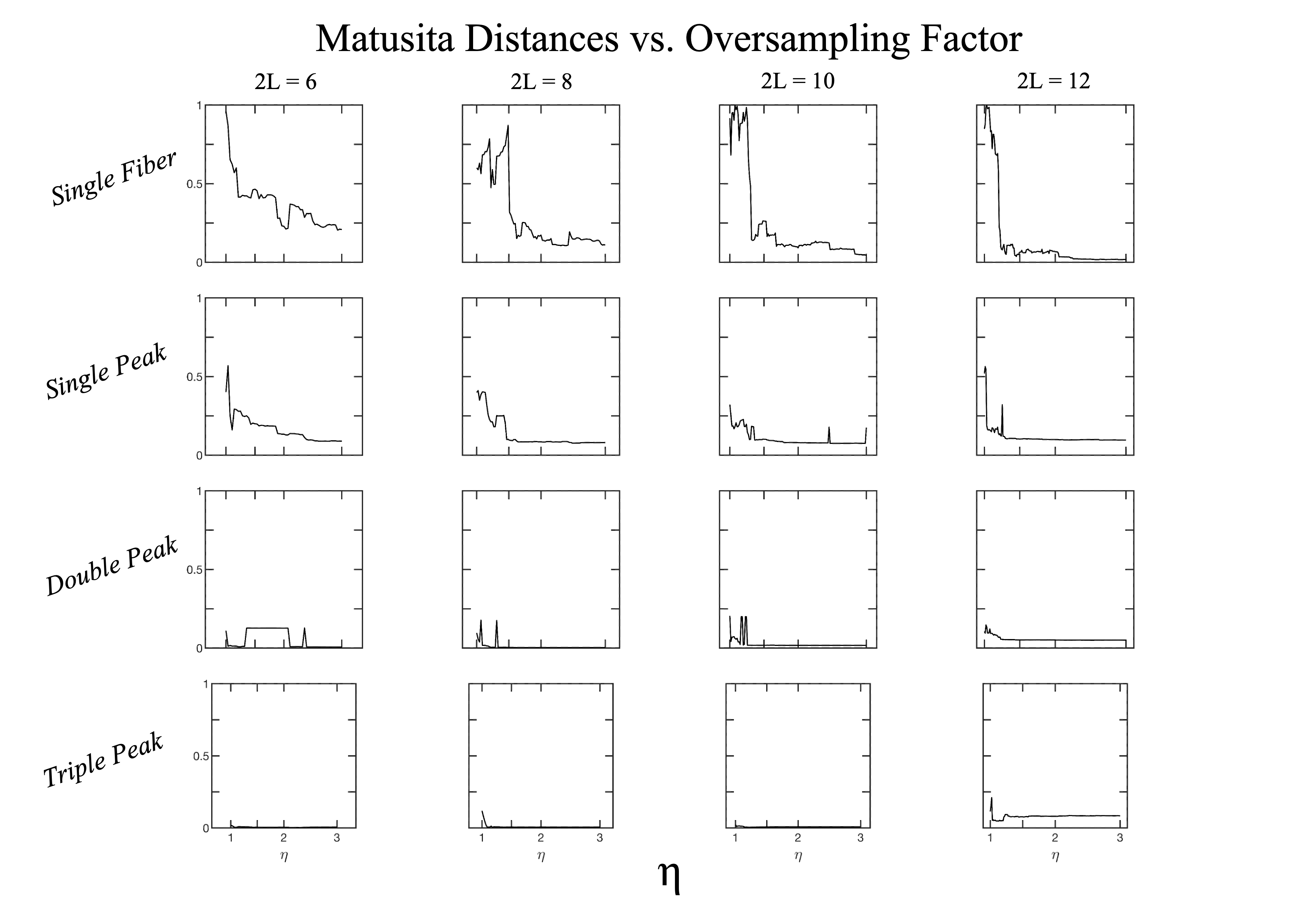
Figure 1 shows the original and approximate fODFs for the single fiber fODF obtained from spherical harmonic expansions with the maximum degree $$$ 2L $$$ varying from 6 to 12. The approximate fODFs were calculated with oversampling factors of $$$ \eta = 1, 1.5, 2,\text{and } 3 $$$. All fODFs were rectified, and only a single hemisphere is displayed. Across all maximum degrees, substantial aliasing errors are apparent in the approximate fODFs for $$$ \eta = 1 $$$, which diminish substantially as $$$ \eta $$$ is increased. Figures 2, 3, and 4 give the corresponding results for the three experimental fODFs. Figure 5 plots the Matusita distances between the approximate and original fODFs as a function of $$$ \eta $$$. In all cases, aliasing errors are seen to be less than 0.31 for $$$ \eta = 1.5 $$$, less than 0.21 for $$$ \eta = 2 $$$, and less than 0.15 for $$$ \eta = 3 $$$.

Discussion and Conclusion

Without some degree of oversampling, fODFs estimated with diffusion MRI can suffer from substantial aliasing errors. However, oversampling by a factor of $$$\eta = 1.5 $$$ already reduces aliasing errors markedly, and these are reduced to low levels for $$$ \eta \ge 2 $$$ in all cases considered. Therefore, oversampling is essential in order to obtain accurate spherical harmonic expansion approximations for fODFs with sharp peaks.

Acknowledgements

This work was supported, in part, by National Institutes of Health grants F31NS108623 and R01AG054159.