3485

Accelerated Echo Planar J-Resolved Spectroscopic Imaging in Prostate Cancer and A Hybrid Dictionary Learning-Total Variation Reconstruction

Ajin Joy¹, Rajakumar Nagarajan¹, Andres Saucedo¹, Zohaib Iqbal¹, Manoj K Sarma¹, Neil E Wilson¹, Ely R Felker¹, Robert E Reiter², Steven S Raman¹, and M Albert Thomas¹
¹Radiological Sciences, University of California-Los Angeles, Los Angeles, CA, United States, ²Urology, University of California-Los Angeles, Los Angeles, CA, United States

Synopsis

Prospectively undersampled 5D echo-planar J-resolved spectroscopic imaging (EP-JRESI) data were acquired in 9 prostate cancer patients and 3 healthy controls. The 5D data was reconstructed using Dictionary learning (DL), Total Variation (TV), Perona-Malik (PM) and a hybrid DLTV method combining DL and TV. DLTV uses the gradient sparsity of TV and the learned dictionary-based sparsity of DL to further increase the transform sparsity of the data. The DLTV method unambiguously resolved 2D J-resolved peaks including myo-inositol, citrate, creatine, spermine and choline with an improved reconstruction that facilitates higher acceleration factors, leading to significant reduction in scan time.

Introduction

Prostate cancer (PCa) is the most common cancer and the second leading cause of cancer mortality in American men (1-2). Magnetic Resonance Spectroscopic Imaging (MRSI), facilitates the acquisition of spectral data from multiple regions of the prostate, from either a selected volume of interest (VOI) or multiple slices (3-5). However, the MRSI total scan duration is very long (3). Therefore, undersampled acquisition followed by compressed sensing (CS) reconstruction is generally employed for the accelerated scan (6). In this work, we have evaluated the performance of a hybrid Dictionary Learning (DL)-Total Variation (TV) (DLTV) reconstruction using non-uniformly sampled (NUS) 5D echo-planar J-resolved spectroscopic imaging (EP-JRESI) data acquired in PCa patients and healthy controls and compared with TV, DL and Perona-Malik (PM) reconstruction techniques (6-10).

Materials and Methods

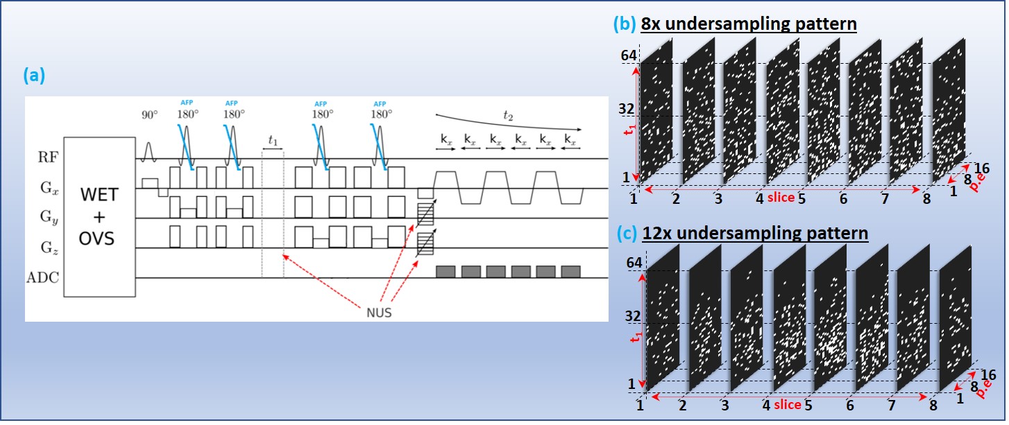
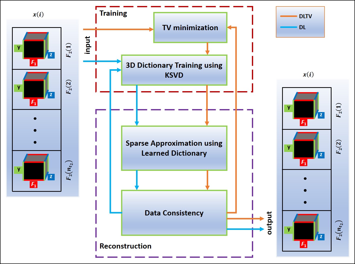
Nine PCa patients (mean age:63years, Gleason scores:6-7, Prostate-specific antigen levels:3-6.9ng/mL) and three healthy males (mean age:42.7years) were investigated, using 3T Siemens MRI scanner with either an endorectal or external phased-array "receive" coil. A maximum echo-based 5D EP-JRESI sequence, as shown in Fig.1(a) (11). The acquisition parameters were: TR/TE/Avg = 1200ms/41ms/1, 16k_x, 16k_y, 8k_z, 512t₂, 64t₁, and voxel resolution = 1x1x1.5cm³. Spectral bandwidths were 1190Hz and ±250Hz for direct and indirect dimensions. An 8x-12x NUS was imposed along t₁, k_yand k_z (Fig.1(b) & (c)). WET-suppression was used for the global suppression of water (12). A fully sampled 5D EP-JRESI scan (TR of 1.5s, 32k_x, 16k_y, 8k_z, 512t₂, 64t₁) of home-made prostate phantom was used for retrospective NUS and CS reconstruction.

Both TV and PM use gradient sparsity for CS reconstruction. DL learns a dictionary using the K-SVD algorithm. The learned set of basis functions achieve a higher sparsity level for the particular signal of interest (13-15). The DLTV combines DL and TV by training dictionaries from a TV filtered data as shown in Fig. 2. Accelerated reconstruction was achieved by operating DLTV in a customized 3D k-space formed by stacking the direct spectral dimension (F₂) (input in Fig.2). This accelerates the reconstruction by training a single dictionary for F₂, instead of separate dictionaries for each F₂ point. The associated cost function minimization is
$$\min_{D,m_f,\rho_\mathscr{R},\rho_\mathscr{I}}\sum_i(\parallel\rho_{\mathscr{R},i}\parallel_0+\parallel\rho_{\mathscr{I},i}\parallel_0)+\mu\mid\triangledown m_f\mid_1+\nu\parallel{F_um_f-s_f}\parallel_2^2 s.t \left\{\begin{array}{cc} \parallel{D\rho_{\mathscr{R},i} -\mathbb{R}_i\mathscr{R}(m_f)}\parallel_2^2<\epsilon\\ \parallel{D\rho_{\mathscr{I},i} -\mathbb{R}_i\mathscr{I}(m_f)}\parallel_2^2<\epsilon\\ \end{array}\right\} \forall i$$ where, $$$s_f$$$ and $$$m_f$$$ are the acquired and reconstructed custom-3D k-space. $$$F_u$$$ computes forward and inverse Fourier transforms in image and temporal domains, and set the values at unacquired locations of k-space as zeros. $$$\mu$$$ and $$$\nu$$$ controls gradient sparsity and data consistency. $$$D$$$ is a real valued, adaptively learnt dictionary. $$$\mathbb{R}$$$ extracts 3D blocks from the custom-3D space and $$$i$$$ is the block number. $$$\rho$$$ is the sparse representation of block. $$$\mathscr{R}$$$ and $$$\mathscr{I}$$$ denotes the real and imaginary components. Normalized-root-mean-squared-error (NRMSE) measure was used to evaluate the reconstruction performance.
$$NRMSE=\dfrac{100}{\sqrt{N_s}}\times\dfrac{\parallel data_R-data_{GT}\parallel_2}{\parallel data_{GT}\parallel_2}$$ where $$$data_{GT}$$$ and $$$data_{R}$$$ are the fully sampled and reconstructed data. $$$N_s$$$ is the number of elements in $$$data_{R}$$$.

Results

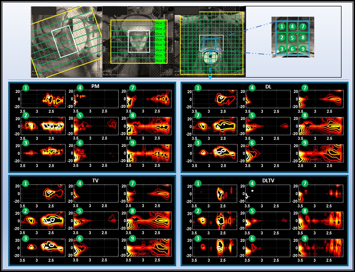
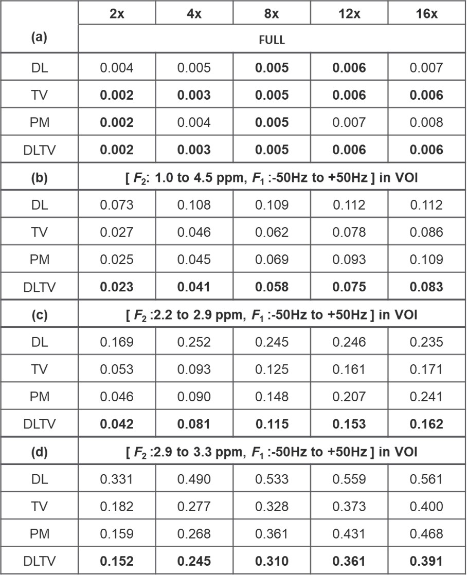
Table 1 lists the NRMSE values of retrospectively undersampled phantom reconstruction. The NRMSE for DL is higher than PM and TV at lower undersampling, and become comparable at higher undersampling levels. DLTV shows lower NRMSE at all acceleration factors considered. Furthermore, 2.9-3.3 ppm range shows higher NRMSE than 2.2-2.9 ppm range. This suggests an overall better reconstruction in the regions with higher SNR. Fig. 3 shows the reconstruction of a prospectively undersampled in-vivo prostate scan (8x) of a 26-year-old healthy volunteer. The spectra show different metabolites including citrate (2.6ppm), creatine (3ppm, 3.9ppm), choline (3.2ppm), myo-inositol (3.5ppm) and Glx (2.2-2.4ppm). While DLTV shows better reproduction of the creatine peak (3.9ppm) that appears to be mixed with myo-inositol/Choline peak (4ppm) in PM, TV and DL. The advantage was more noticeable in Fig. 4 that showed the reconstruction at 12x acceleration (8.33% k-space samples were collected from a 48-year-old PCa patient (Gleason score of 4+3)). DLTV was able to differentiate creatine and choline peaks at 3 and 3.2 ppm in voxels numbered 8 and 9, better than other methods. While voxels 5 and 6 show depleted citrate across all four reconstructions indicating cancerous location, none of the methods manage to distinguish the choline peak at 3.2 ppm as good as DLTV.

Discussion

Better reconstruction of the 5D data was possible using the combination of DL and TV in DLTV compared to DL and TV alone. This can be understood based on the fact that the effectiveness of DL is also dependent on the quality of training data. The TV-filtered training data therefore helps DL to find a better sparse representation, leading to an overall improved performance. Thus, the additional TV filtering step allows for potentially higher undersampling factors (8), which can lead to further reductions in scan time without overly compromising the data quality.

Conclusion

The hybrid DLTV reconstruction technique, which considers the data to be sparse in both learned basis and in the finite difference-based representation, can facilitate higher undersampling rates for MRSI scans. This approach can help to bring down the total scan time of a 5D EP-JRESI scan from 21 minutes to 14 minutes by using 12x undersampling factor instead of 8x for a TR of 1.2ms on a 16×16×8 cartesian sampling grid.

Acknowledgements

Authors acknowledge the support by a CDMRP grant from the US Army Prostate Cancer Research Program: (#W81XWH-11-1-0248) and NIH (P50CA092131, 5R21MH125349, 5R01HL135562).

References

1. About prostate cancer. https://www.cancercenter.com/cancer-types/prostate-cancer/about. Accessed on Nov 1,2021.

2. Maier SE, Walstrom J, Langklide F, Johansson J, Kuczera S, Hugosson J, Hellstrom M. Prostate cancer diffusion-weighted magnetic resonance imaging : Does the choice of diffusion-weighting level matter ?. J Magn Reson Imaging 2021 Sep.18

3. Bogner W, Otazo R, Henning A.Bogner W, et al. Accelerated MR spectroscopic imaging-a review of current and emerging techniques. NMR Biomed. 2021 May;34(5): e4314. Epub 2020 May 12.

4. Maudsley AA, Andronesi OC, Barker PB, Bizzi A, Bogner W, Henning A, Nelson SJ, Posse S, Shungu DC, Soher BJ, Maudsley AA, et al. Advanced magnetic resonance spectroscopic neuroimaging: Experts' consensus recommendations. NMR Biomed. 2021 May;34(5):e4309. Epub 2020 Apr 29.

5. Kurhanewicz J, Vigneron D, Hricak H, Narayan P, Carroll P and Nelson SJ, Three dimensional H-1 MR Spectroscopic Imaging of the in situ human prostate with high (0.24-0.7cm3) spatial resolution, Radiology 1996; 198:795-805.

6. Furuyama J, Wilson N, Burns B, Nagarajan R, Margolis D and Thomas MA. Application of Compressed Sensing to Multidimensional Spectroscopic Imaging in Human Prostate. Magn Reson Med 2012;67:1499-1505, April 13

7. Joy A, Paul JS. Multichannel compressed sensing MR image reconstruction using statistically optimized nonlinear diffusion. Magn Reson Med 2017;78(2):754-762.

8. Ravishankar S, Bresler Y. MR image reconstruction from highly undersampled k-space data by dictionary learning. IEEE transactions on medical imaging. 2010;30(5):1028-41.

9. Joy A, Jacob M and Paul, JS. Compressed sensing MRI using an interpolation‐ free nonlinear diffusion model. Magn Reson Med 2021;85(3):1681-1696.

10. Nagarajan R, Iqbal Z, Burns B, Wilson NE, Sarma MK, Margolis DA, Reiter RE, Raman SS, Thomas MA. Accelerated echo planar J-resolved spectroscopic imaging in prostate cancer: a pilot validation of non-linear reconstruction using total variation and maximum entropy. NMR Biomed. 2015 Nov;28(11):1366-73.

11. Wilson NE, Iqbal Z, Burns BL, Keller M and Thomas MA. Accelerated five dimensional echo planar J-resolved spectroscopic imaging: Implementation and pilot validation in human brain. Magn Reson Med 2016;75:42-51. Epub 2015 Jan.19.

12. Ogg RJ, Kingsley RB and Taylor JS. WET, a T1-and B1-insensitive water-suppression method for in vivo localized 1H NMR spectroscopy. JMagn Reson, Series B, 1994;104(1):1-10.

13. Aharon M, Elad M, Bruckstein A. K-SVD: An algorithm for designing overcomplete dictionaries for sparse representation. IEEE Trans Sig Processing. 2006;54(11):4311-22.

14. Rubinstein R, Bruckstein AM, Elad M. Dictionaries for sparse representation modeling. Proceedings of the IEEE. 2010;98(6):1045-57.

15. Liu Q, Wang S, Ying L, Peng X, Zhu Y, and Liang D. Adaptive dictionary learning in sparse gradient domain for image recovery. IEEE Trans Image Processing. 2013;22(12):4652-4663.

Figures

Figure 1: (a) Schematics diagram of the 5D NUS EPJRESI pulse sequence. An example of nonuniform sampling pattern based on exponentially decaying probability density for (a) 8x undersampling and (c) 12x undersampling is shown. White and black colors represent acquired and unacquired locations in the k-space.

Figure 2: Comparison of DL and DLTV workflow. Yellow and blue colored arrows represent DL and DLTV workflow respectively. y, z and F₁ represents the Fourier transform of k_y, k_z and t₁ after filling the missing samples with zeros. F₂ and x are the Fourier transforms of fully sampled t₂ and k_x dimensions.

Figure 3: Reconstruction of the prospectively undersampled (8x) 5D EP-JRESI data acquired in a 26-year-old healthy volunteer. Localization images are shown in the top-left panel. Bottom panel shows the distribution of spectra (F₂: 2 to 4.5ppm, F₁: -25 to +25Hz) within the blue bounding box. The 2D spectra show different metabolites including citrate, creatine, choline, spermine, myo-Inositol and Glx. Individual voxels are labeled from 1 to 4 using green circles. An enlarged view of the DLTV reconstruction of voxel 3 with labeled metabolites is shown on the top-right panel.

Figure 4: Reconstruction of the prospectively undersampled (12x) 5D EP-JRESI data acquired in a 48-year-old patient (Gleason score of 4+3). Localization images of sagittal, coronal and axial planes are shown in the top panel. Bottom panel shows the distribution of spectra (F₂: 2 to 3.6ppm, F₁: -25 to +25Hz) within the blue bounding box in VOI (white bounding box), reconstructed using PM, TV, DL and DLTV. Individual voxels are labeled from 1 to 9 using green circles.

Table 1: NRMSE comparison of PM, TV, DL and DLTV reconstruction of prostate phantom data retrospectively undersampled at 2x, 4x, 8x, 12x and 16x. (a) NRMSE in the full range of spectrum, across all voxels. (b) NRMSE in the voxels within VOI in the range of 1 to 4.5 ppm along F₂ and -50 to +50 Hz along F₁ dimensions. (c) NRMSE values within VOI in the range of 2.2 to 2.9 ppm along F₂ and -50 to +50 Hz along F₁ dimension. (d) NRMSE values within VOI in the range of 2.9 to 3.3 ppm along F₂ and -50 to +50 Hz along F₁ dimension.

Proc. Intl. Soc. Mag. Reson. Med. 30 (2022)

3485

DOI: https://doi.org/10.58530/2022/3485