3483
Polynomial Preconditioning for Accelerated Convergence of Proximal Algorithms including FISTA1Department of Electrical Engineering and Computer Science, Massachusetts Institute of Technology, Cambridge, MA, United States, 2Department of Radiology, Stanford University, Stanford, CA, United States, 3Department of Electrical Engineering, Stanford University, Stanford, CA, United States
Synopsis
This work aims to accelerate the convergence of proximal gradient algorithms (like FISTA) by designing a preconditioner using polynomials that targets the eigenvalue spectrum of the forward linear model to enable faster convergence. The preconditioner does not assume any explicit structure and can be applied to various imaging applications. The efficacy of the preconditioner is validated on four varied imaging applications, where it seen to achieve 2-4x faster convergence.
Introduction
Since the introduction of compressed sensing MRI[1], iterative proximal methods[2] have emerged as the workhorse algorithms used to solve MRI reconstruction, commonly posed as the minimization of the sum of a smooth, least-squares data-consistency cost (denoted $$$f$$$) and a possibly non-smooth regularization (denoted $$$g$$$) with an easily computable proximal operator.$$\text{Equation 1: } F(x) = f(x) + g(x) \text{ where } f(x) = \frac{1}{2}\lVert Ax - b\rVert_2^2$$
Here, $$$A$$$ is a linear function that models how the underlying signal $$$x$$$ gets mapped to the acquired data $$$b$$$.
The above is best solved by the Fast Iterative Shrinkage-Thresholding Algorithm (FISTA)[3] which enjoys theoretically optimal guarantees. However, in practice, the convergence of iterative proximal methods is limited by the conditioning of $$$f$$$ as determined by the eigenvalues of $$$A^*A$$$.
This work aims to alleviate this issue by designing a preconditioner that targets the spectrum of $$$A^*A$$$ to enable faster convergence. The proposed preconditioner is derived directly from $$$A^*A$$$ without assuming any explicit structure of $$$A$$$, and thus can be applied to various imaging applications that satisfy certain natural conditions. Since the preconditioner is derived from $$$A^*A$$$, it also does not require any additional computational resources compared to PGD or FISTA. The efficacy of the preconditioner is validated on four varied imaging applications, where it seen to achieve 2-4x faster convergence.
Theory
DerivationFor simplicity, this work analyses proximal gradient descent (PGD)[2] and assumes $$$A^*A$$$ is full-rank. Without loss of generality, assume the eigenvalues of $$$A^*A \subset (0, 1]$$$. Let $$$\text{prox}_g$$$ be the proximal operator of $$$g$$$. (For $$$g = \lambda \lVert x \rVert_1$$$, the proximal operator corresponds to soft-thresholding using $$$\lambda$$$.) PGD can be used to solve Equation 1 as follows:
$$\text{Equation 2: } x_{k+1} = \text{prox}_g(x_k - A^*(Ax_k - b))$$
Here, $$$x_k$$$ denotes the $$$k^{th}$$$ iterand. Let $$$x_\infty = \lim_{k\rightarrow\infty}x_k$$$ be the final converged solution. By the fixed-point property of proximal operators[2]:
$$\text{Equation 3: } x_\infty = \text{prox}_g(x_\infty - A^*(Ax_\infty - b))$$
Taking the $$$l_2-$$$norm of the difference between Equation 2 and Equation 3, the firm none-expansiveness property of proximal operators[2] yields:
$$\text{Equation 4: } \lVert x_{k+1} - x_\infty \rVert_2 < \lVert (I - A^*A) (x_{k} - x_\infty)\rVert_2$$
The strict inequality comes from the assumption that $$$A^*A$$$ is full-rank. Equation 4 shows that the convergence of PGD is determined by the magnitudes of the eigenvalues of $$$I - A^*A$$$. That is to say, the component of the error vector $$$(x_{k+1}-x_\infty)$$$ corresponding to an eigenvalue $$$\lambda$$$ of $$$A^*A$$$ decreases in norm by $$$|1 - \lambda|$$$ after an iteration. Consequently, the small eigenvalues of $$$A^*A$$$ have $$$|1 - \lambda|\approx1$$$, resulting in slow convergence.
Instead of the PGD update step in Equation 2, this work proposes adding a preconditioner $$$P$$$ to the update step:
$$\text{Equation 5: } y_{k+1} = \text{prox}_g(y_k - PA^*(Ay_k - b)) \text{ where } P = p(A^*A)$$
The iteration variable name has been changed to reflect which algorithm is being used. $$$p$$$ is a designed polynomial that will be defined in the sequel. With the preconditioner, the error terms decay as:
$$\text{Equation 6: } \lVert y_{k+1} - y_\infty \rVert_2 < \lVert (I - P A^*A) (y_{k} - y_\infty)\rVert_2$$
Consequently, $$$P = p(A^*A)$$$ can be designed to bring the eigenvalues of $$$I - PA^*A$$$ as close to zero as possible. Thus:
$$\text{Equation 7: }\left\{\begin{array}{rcl}c&=&\underset{c_0,c_1,\dots,c_d}{\text{argmin}}\int_{z=0}^1|1-(c_0+c_1z+c_2z^2+\dots+c_dz^d)z|^2dz\\p(z)&=&c_0+c_1z+c_2z^2+\dots+c_dz^d\\P&=&p(A^*A)\\&=&c_0I+c_1A^*A+c_2(A^*A)^2+\dots+c_d(A^*A)^d\end{array}\right.$$
From Equation 6, the component of $$$y_k - y_\infty$$$ corresponding to eigenvalue $$$\lambda$$$ now is scaled by $$$|1-p(\lambda)\lambda|$$$. Since prior knowledge of the eigenvalue distribution is not known, Equation 7 minimizes over the entire spectrum of the eigenvalues of $$$A^*A$$$.
Note that Equation 5 solves a slightly different optimization problem than Equation 1. It is possible to show that for applications where the data-consistency cost of the final solution is small (i.e., $$$\lVert Ax_\infty - b \rVert < \epsilon$$$), then $$$\lVert x_\infty - y_\infty \rVert \sim O(\epsilon)$$$ (i.e., Equation 5 yields almost exactly the same solution as Equation 2.)
The degree of the polynomial $$$p$$$ is fixed so that Equation 7 can be solved easily. The degree is a hyper-parameter that is to be tuned for the desired application.
Computation
Assuming $$$p$$$ is of degree $$$d$$$, note that one iteration of Equation 5 has the same number of $$$A^*A$$$ evaluations as $$$(d+1)$$$ iterations of Equation 2. However, the main benefit of the preconditioner is that for comparable computational effort, it is possible to explicitly target the smaller eigenvalues of $$$A^*A$$$. This is demonstrated in Figure 1.
Methods & Results
All the following experiments were implemented in SigPy[4] and performed using an NVIDIA(R) 1080 Ti with 1 CPU thread for reproducibility. Please see Figure 2,3,4 and 5 for experiment details and results with wall-times reported.Discussion
The preconditioner is demonstrated to achieve 2-4x faster convergence on 4 varied applications of interest. By targeting the smaller eigenvalues of $$$A^*A$$$, the finer details of the underlying signal are resolved quicker. The preconditioner easily extends to subspace reconstructions for spatiotemporal applications as demonstrated in Figure 4 and Figure 5, thus scaling well with problem-size, unlike in k-space diagonal preconditioning for the primal-dual hybrid-gradient algorithm[5]. Additionally, since the preconditioner is derived from $$$A^*A$$$, applications with a fast normal operators such as T2-Shuffling[6] and the Toeplitz PSF[7] can be leveraged.The polynomial optimization in Equation 7 was also utilized to accelerate conjugate gradient for least squares[8]. This work extends the principle to proximal algorithms.
Acknowledgements
This study is supported in part by GE Healthcare research funds and NIHnR01EB020613, R01MH116173, R01EB019437, U01EB025162 , P41EB030006.References
- Lustig, Michael, et al. "Compressed sensing MRI." IEEE signal processing magazine 25.2 (2008): 72-82.
- Parikh, Neal, and Stephen Boyd. "Proximal algorithms." Foundations and Trends in optimization 1.3 (2014): 127-239.
- Beck, Amir, and Marc Teboulle. "A fast iterative shrinkage-thresholding algorithm for linear inverse problems." SIAM journal on imaging sciences 2.1 (2009): 183-202.
- Ong, Frank, and Michael Lustig. "SigPy: a python package for high performance iterative reconstruction." Proceedings of the International Society of Magnetic Resonance in Medicine, Montréal, QC 4819 (2019).
- Ong, Frank, Martin Uecker, and Michael Lustig. "Accelerating non-Cartesian MRI reconstruction convergence using k-space preconditioning." IEEE transactions on medical imaging 39.5 (2019): 1646-1654.
- Tamir, Jonathan I., et al. "T2 shuffling: sharp, multicontrast, volumetric fast spin‐echo imaging." Magnetic resonance in medicine 77.1 (2017): 180-195.
- Baron, Corey A., et al. "Rapid compressed sensing reconstruction of 3D non‐Cartesian MRI." Magnetic resonance in medicine 79.5 (2018): 2685-2692.
- Johnson, Olin G., Charles A. Micchelli, and George Paul. "Polynomial preconditioners for conjugate gradient calculations." SIAM Journal on Numerical Analysis 20.2 (1983): 362-376.
- Jiang, Yun, et al. "MR fingerprinting using fast imaging with steady state precession (FISP) with spiral readout." Magnetic resonance in medicine 74.6 (2015): 1621-1631.
- Cao, Xiaozhi, et al. "Robust sliding‐window reconstruction for Accelerating the acquisition of MR fingerprinting." Magnetic resonance in medicine 78.4 (2017): 1579-1588.
- Wang, Fuyixue, et al. "3D Echo Planar Time-resolved Imaging (3D-EPTI) for ultrafast multi-parametric quantitative MRI." bioRxiv (2021).
- Wang, Fuyixue, et al. "Echo planar time‐resolved imaging (EPTI)." Magnetic resonance in medicine 81.6 (2019): 3599-3615.
- Dong, Zijing, et al. "Echo planar time‐resolved imaging with subspace reconstruction and optimized spatiotemporal encoding." Magnetic resonance in medicine 84.5 (2020): 2442-2455.
Figures
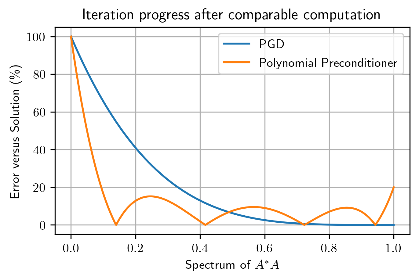
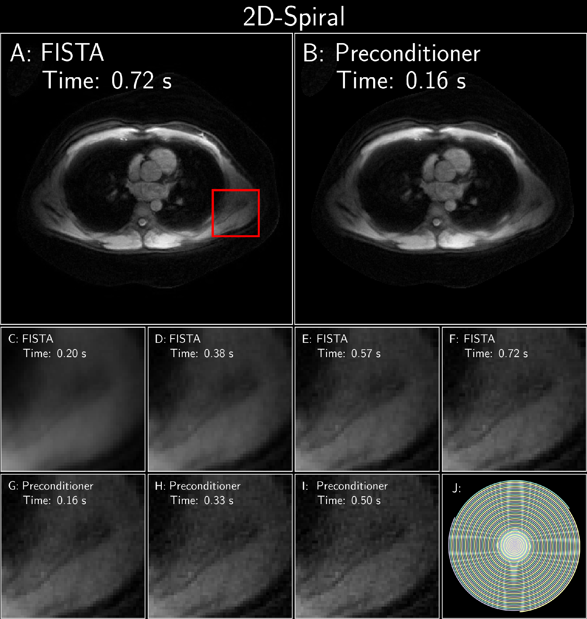
Figure 2: FISTA with and without an optimized polynomial preconditioner of degree 7 on a cardiac dataset (available at https://github.com/mikgroup/kspace_precond[5]). Acquisition: Variable density spiral
trajectory; 1.5T scanner (GE Healthcare, Waukesha, WI); 8-channel cardiac coil and the HeartVistaRTHawk platform (HeartVista,
Los Altos, CA). Trajectory: 3 interleaves; 3996
readout points; effective under-sampling=8. FOV=32x32 cm2. matrix size=320x320. TR=25.8ms. Both recons used a sparse Wavelet prior. J: sampling pattern.
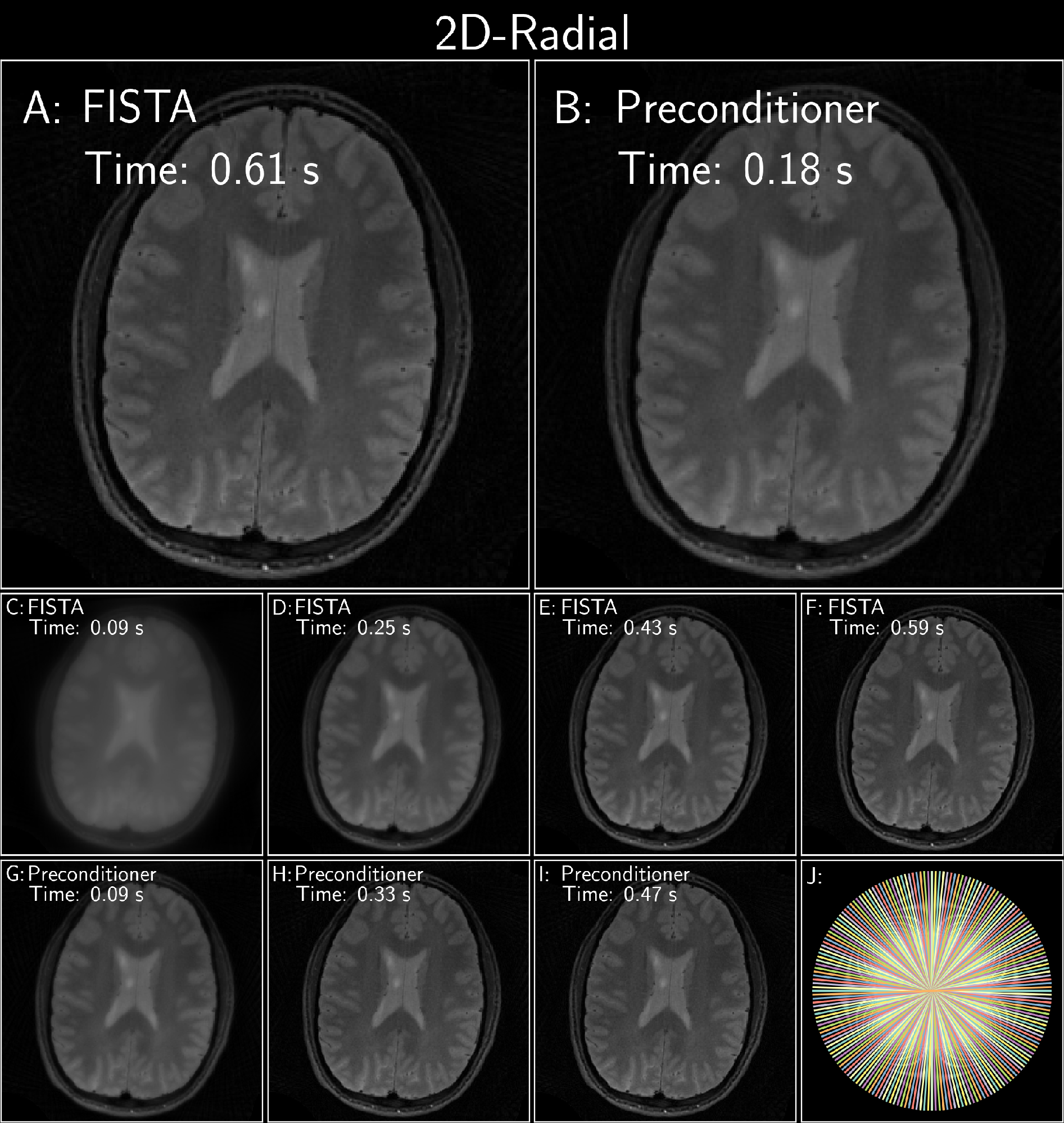
Figure 3: FISTA with and without an optimized polynomial preconditioner of degree 8 on a radial brain dataset (12 receive channels, 96 radial projections) from the ISMRM reproducibility challenge (available at available at https://github.com/mikgroup/sigpy-mri-tutorial[4]). Both reconstructions used a sparse Wavelet prior. (J) shows the under-sampling pattern.
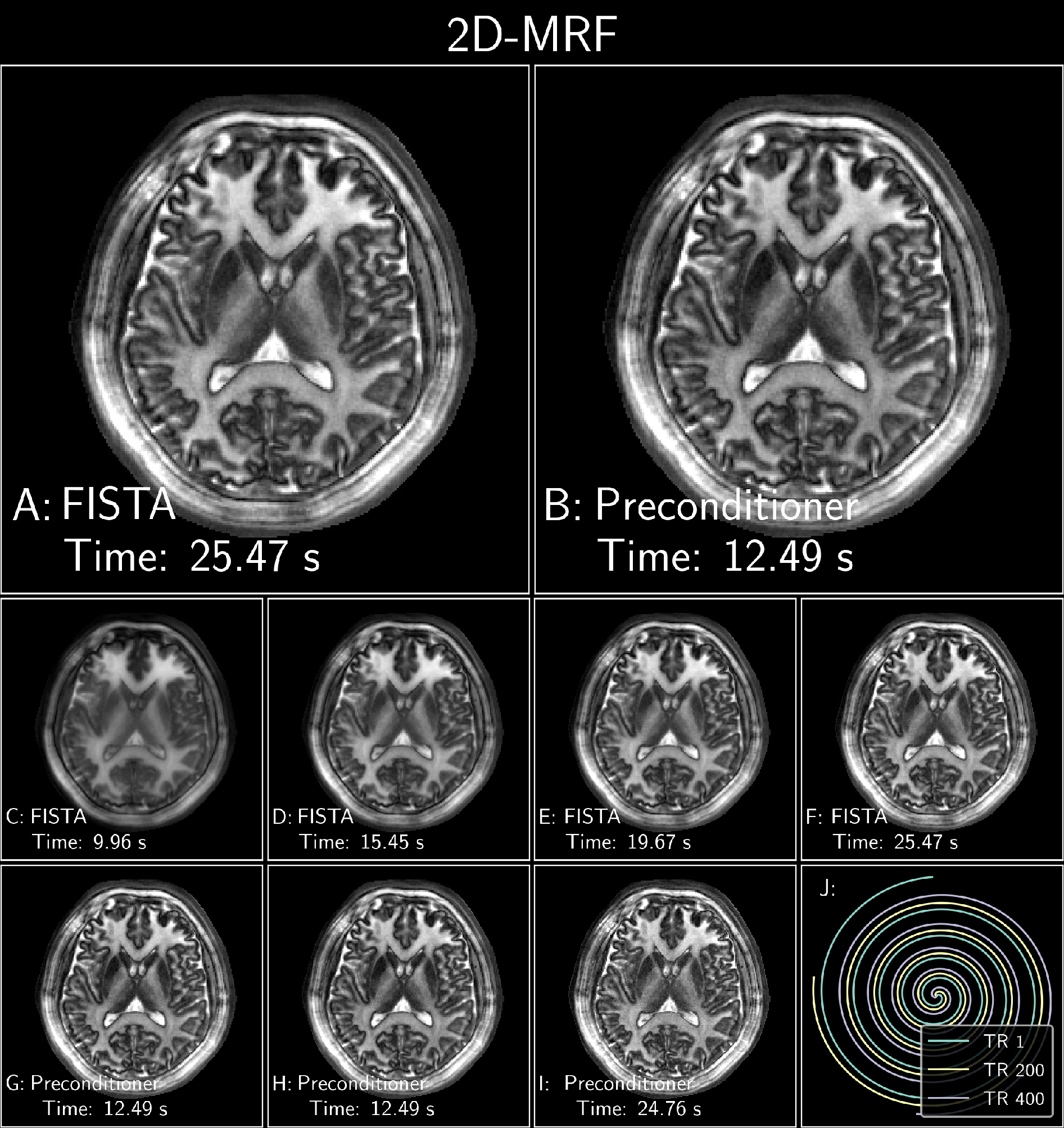
Figure 4: FISTA with and without an optimized polynomial preconditioner of degree 8 applied to a 2D Spiral MRF subspace reconstruction with locally low-rank[9,10]. The data was acquired on 3T Premier scanner using a 48-channel head coil (GE Healthcare, Waukesha, WI) with 500 spiral interleaves, 1688 readout points, 500 TRs, 5mm slice thickness, TE=1.5ms, TR=15ms, FOV=220x220mm2 at 1mm in-plane resolution. The temporal subspace was of rank 5. For succinctness, only the 3rd coefficient is shown. J: Subset of spirals demonstrating the sampling pattern.

Figure 5: FISTA with and without a polynomial preconditioner of degree 8 applied to a subspace 3D-EPTI reconstruction with locally low-rank[11,12,13]. Data obtained from https://github.com/Fuyixue/3D-EPTI. The data was Fourier transformed along the readout and a single slice was used. The data has 1490 echoes and each echo had 29 sampled (ky, kz) points. The temporal basis was rank of 12; reconstruction size was: 120x150; and the acquired resolution was 1.5x1.5mm2. For succinctness, only the 2nd coefficient is displayed.