3478
K-space refinement method for DL-based MR reconstruction by regularizing k-space null space constraint with auto-calibrated kernel1Radiology, Stanford University, Stanford, CA, United States, 2Electrical Engineering, Stanford, Stanford, CA, United States
Synopsis
In this study, we propose a novel refinement method using auto-calibrated k-space null-space kernel to reduce the k-space errors and enable reconstruction of improved high-frequency image details and textures. The refinement algorithm can be easily plugged in after DL-based reconstructions. We show that our method enables the reconstruction of sharper images with significantly improved high-frequency components measured by HFEN and GMSD while maintaining overall error in the image measured by PSNR and SSIM.
Introduction
Deep Learning (DL) based reconstruction using unrolled neural networks has shown great potential in accelerating magnetic resonance imaging (MRI) [1-2]. However, one of the major drawbacks is the loss of high-frequency details and textures in the output [3-4].In this work, we propose a novel refinement method using auto-calibrated k-space null-space kernel [ref] to reduce the k-space errors and enable reconstruction of improved high-frequency image details and textures. The proposed scheme constrains the DL output to satisfy the neighborhood relationship in the frequency space (k-space) which can be easily calibrated in the auto-calibration (ACS) lines, and corrects the under-estimation in the peripheral region of the k-space as well as reduce structured k-space errors. Note that auto-calibrated k-space null space kernel contains additional information such as coil sensitivities, image features, limited spatial support, slowly varying phase, and etc [5-8].
We show that our method enables the reconstruction of sharper images with significantly improved high-frequency components measured by HFEN [9] and GMSD [10] while maintaining overall error in the image measured by PSNR and SSIM.
Methods
DatasetFor this study, we used the “Brain dataset” (T1 post contrast enhanced), and the “Knee dataset” (with proton density weighted + proton density weighted with fat suppression). For the Brain dataset, we used the dataset marked as “validation” which we split the data randomly into (Train=212, Val=32, Test=42 subjects). For the Knee dataset, we split the data into (Train=108, Val=30, Test=62 subjects). For both dataset, equi-spaced undersampling (R=4,6) were used for the work.
DL Networks for MR reconstruction
Two state-of the art unrolled neural networks were used – Variational Network [ref], MoDL [ref]. For Variational Network (VarNet) we used 12 unrolled blocks, and MoDL with 10 unrolled block.
Auto-calibrating null-space kernel
For the examples in the study, we used SPIRiT [5] with virtual coil conjugate augmentation [11] as the method for calibrating the null-space kernel. We also tested SURE-based ESPIRiT method for the null-space kernel [7], which offers faster convergence but lacks information of the slowly varying phase.
Proposed refinement:
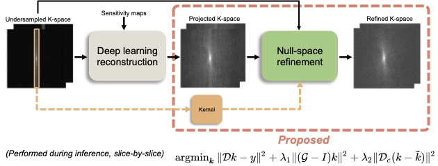
The proposed refinement requires three inputs: acquired under-sampled k-space, null-space kernel that is calibrated from the ACS-line of the undersampled k-space, and the DL reconstructed k-space. The overall scheme of the proposed refinement method and inputs required for the refinement are demonstrated in Fig.1.
With these inputs, we solve the following optimization problem:
$$\operatorname{argmin}_{\boldsymbol{k}}\|\mathcal{D} k-y\|^{2}+\lambda_1\|(\mathcal{G}-I) k\|^{2} + \lambda_2\|\mathcal{D}_c (k - \tilde{k})\|^{2}$$
Where $$$\mathcal{D}_c$$$ is an operator that selects un-acquired k-space locations, $$$\mathcal{G}-I$$$ auto-calibrated null-space kernel, $$$\tilde{k}$$$ the DL-estimated k-space, assuming that the DL estimation has estimated k-space with some degree of precision in mean squared error. For solving the optimization problem, we used the conjugate gradient (CG) algorithm with 300 iterations to ensure convergence.
Results
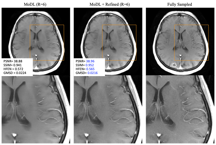
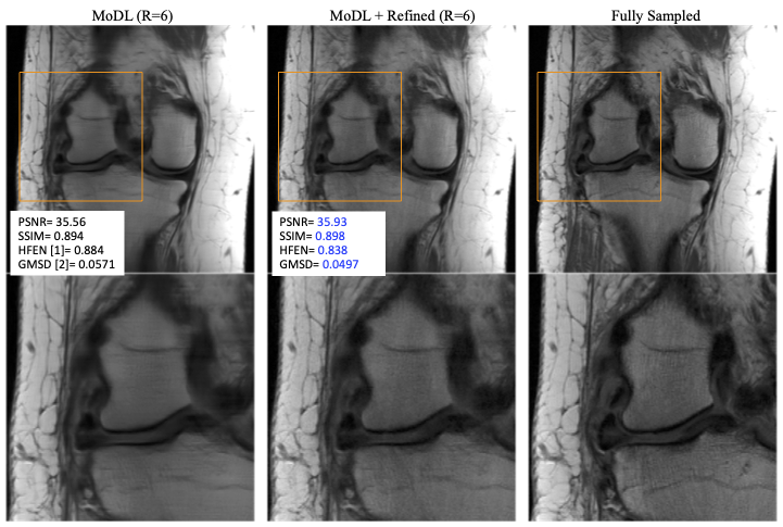
Figure 2 shows the result of refinement on a Brain T1-Post data. First column is a result reconstructed from MoDl with R=6. Second column is the corresponding refinement result, and third column is the reference image from fully sampled k-space. The vessels looks sharper and texture more natural on the refinement results. Quantitative metrics are improved, and specifically HFEN and GMSD (metrics for high-frequency error) show improvements.Figure 3 shows the result of refinement on a PDw knee dataset. First column is a result reconstructed from MoDl with R=6. Second column is the corresponding refinement result, and third column is the reference image from fully sampled k-space. Likewise, sharper details in the ligament and improved texture can be observed.
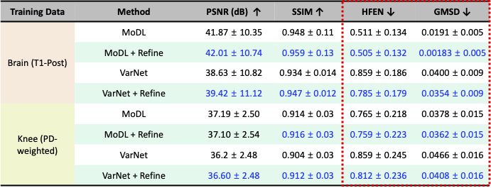
Figure 4 shows the results of quantitative evaluation for acceleration factor of 6. The quantitative metrics are improved with the refinement for both DL methods (VarNet, MoDL).
Conclusions
In this study, we propose a refinement algorithm for recovering texture and details from the DL-based reconstruction. The refinement algorithm can be easily plugged in after DL-based reconstructions. Further works will include -- investigation of using the null-space kernel in the unrolled neural network and applying for higher dimension MR acquisition such as 3D or Cine.Acknowledgements
NIH R01 EB009690, NIH R01 EB026136, and GE HealthcareReferences
[1] K. Hammernik, T. Klatzer, E. Kobler, M. P. Recht, D. K. Sodickson, T. Pock, and F. Knoll, “Learning a variational network for reconstruction of accelerated MRI data,” Magnetic Resonance in Medicine, vol. 79,no. 6, pp. 3055–3071, 2018.
[2] H. K. Aggarwal, M. P. Mani, and M. Jacob, “MoDL: Model-Based Deep Learning Architecture for Inverse Problems,” IEEE Transactions on Medical Imaging, vol. 38, no. 2, pp. 394–40
[3] F. Knoll, T. Murrell, A. Sriram, N. Yakubova, J. Zbontar, M. Rabbat,A. Defazio, M. J. Muckley, D. K. Sodickson, C. L. Zitnick, and M. P. Recht, “Advancing machine learning for MR image reconstruction with an open competition: Overview of the 2019 fastMRI challenge,” Magnetic Resonance in Medicine, vol. 84, no. 6, pp. 3054–3070, 2020.
[4] M. J. Muckley, B. Riemenschneider, A. Radmanesh, S. Kim, G. Jeong,J. Ko, Y. Jun, H. Shin, D. Hwang, M. Mostapha, S. Arberet, D. Nickel,Z. Ramzi, P. Ciuciu, J.-L. Starck, J. Teuwen, D. Karkalousos, C. Zhang, A. Sriram, Z. Huang, N. Yakubova, Y. W. Lui, and F. Knoll, “Results of the 2020 fastMRI Challenge for Machine Learning MR Image Reconstruction,” IEEE Transactions on Medical Imaging, vol. PP, no. 99,pp. 1–1, 20
[5] M. Lustig and J. M. Pauly, “SPIRiT: Iterative self-consistent parallel imaging reconstruction from arbitrary k-space,” Magnetic Resonance in Medicine, vol. 64, no. 2, pp. 457–47
[6] J. P. Halder, “Autocalibrated Loraks for Fast Constrained MRI Reconstruction,” 2015 IEEE 12th International Symposium on Biomedical Imaging (ISBI), pp. 910–913, 2
[7] M. Uecker, P. Lai, M. J. Murphy, P. Virtue, M. Elad, J. M. Pauly, S. S. Vasanawala, and M. Lustig, “ESPIRiT- an eigenvalue approach to autocalibrating parallel MRI: Where SENSE meets GRAPPA,” Magnetic Resonance in Medicine, vol. 71, no. 3, pp. 990–10
[8] J. P. Haldar and J. Zhuo, “P-LORAKS: Low-rank modeling of local k-space neighborhoods with parallel imaging data,”Magnetic Resonancein Medicine, vol. 75, no. 4, pp. 1499–15
[9] S. Ravishankar and Y. Bresler, “MR Image Reconstruction from Highly Undersampled k-Space Data by Dictionary Learning,” IEEE Transactions on Medical Imaging, vol. 30, no. 5, pp. 1028–1041, 2011.
[10] A. Mason, J. Rioux, S. E. Clarke, A. Costa, M. Schmidt, V. Keough,T. Huynh, and S. Beyea, “Comparison of Objective Image Quality Metrics to Expert Radiologists’ Scoring of Diagnostic Quality of MR Images,” IEEE Transactions on Medical Imaging, vol. 39, no. 4, pp.1064–1072
[11] M. Blaimer, M. Gutberlet, P. Kellman, F. A. Breuer, H. K ̈ostler, and M. A. Griswold, “Virtual coil concept for improved parallel MRI employing conjugate symmetric signals,” Magnetic Resonance in Medicine,vol. 61, no. 1, pp. 93–10
Figures