Introduction

MRF¹ is an imaging technique that offers quantification of multiple tissue parameters via a single MRI signal acquisition. Previously, supervised neural networks² have been trained to act as inverse models that predict quantitative tissue parameters from MRF signals. However, this supervised technique relies on comparing predictions to discretized ground truths. These ground truths can be difficult to obtain, especially as the number of tissue parameters of interest increases. We propose the addition of a physics-informed forward model to create a self-supervised³ training loop independent of the need for a ground truth to teach the inverse model neural network.

Methods

MRF data simulation
T1, T2, and proton density (M0) quantitative parameter maps are obtained from multi-slice 2D MRF scans of five healthy subjects. A total of 58 2D brain slices are used to simulate time evolutions of a MRF-FISP scan with 480 time points via the Bloch equations. The flip angles and TR are based on an automated sequence design⁴. The simulated signal is normalized against its maximum absolute value across the entire training dataset such that the normalized signal is bounded by the range [-1,1] to improve network learning.

Model architecture
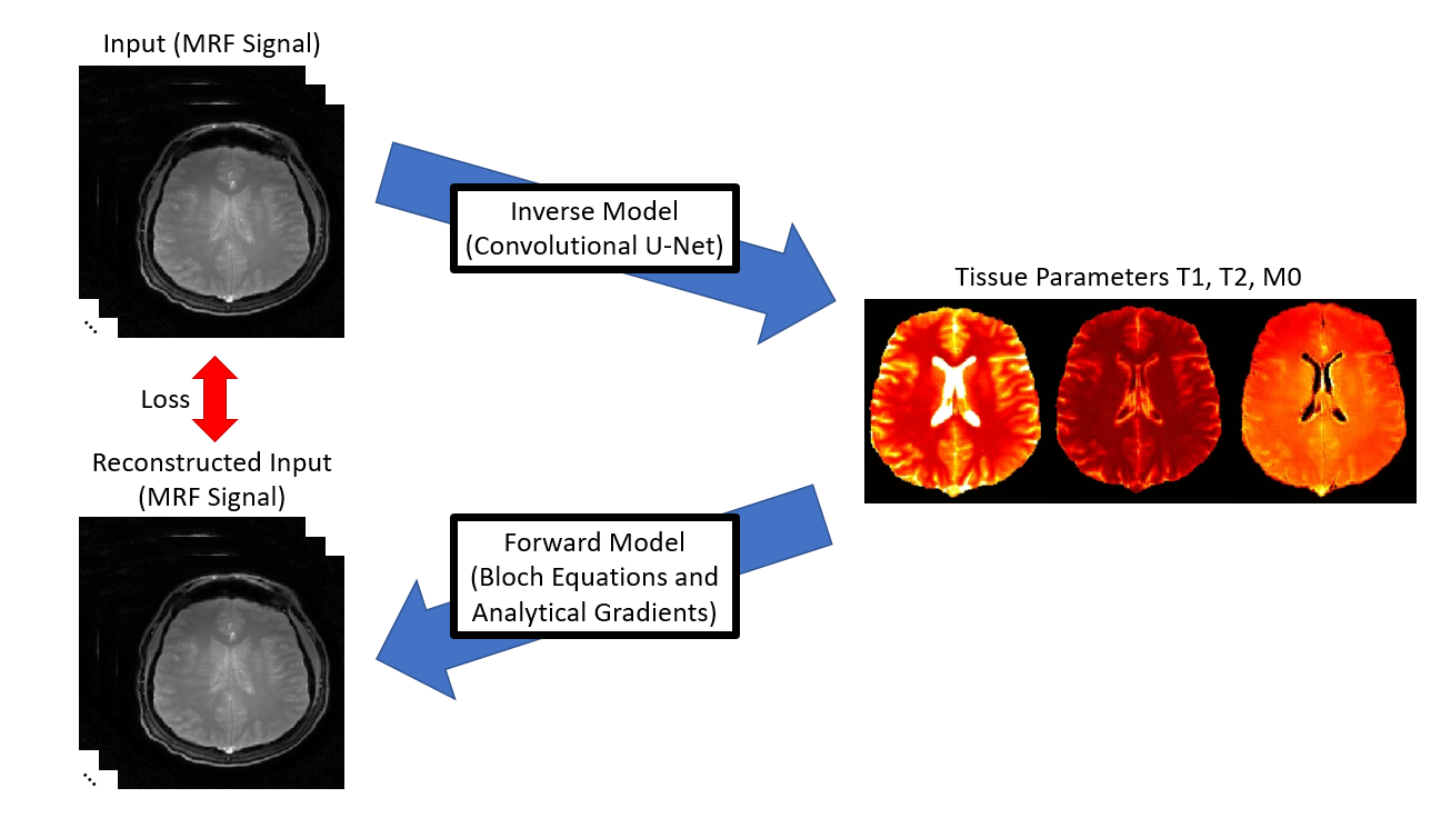
The self-supervised model consists of two halves: the inverse model, which takes a simulated signal and predicts T1, T2, and M0 tissue parameters, and the forward model, which uses a physical model to reconstruct the signal’s time evolution given the predicted tissue parameters from the network. Thus, the model both takes in and outputs time-domain signal data, such that an L1-norm loss can be computed from direct comparison of the two without the need for a ground truth of tissue parameters. This loss is analytically back-propagated through the forward model via the chain rule, such that the gradient dLoss/dParameter is found. From there, Pytorch’s Autograd feature is utilized to update the inverse network’s convolutional weights and biases based on the computed gradient. This network architecture is summarized in figure 1.The inverse model is a convolutional u-net that accepts a number of input channels equal to the time points in the signal evolution and outputs a number of channels corresponding to the tissue parameters of interest. By convolving neighboring pixels, each pixel’s predicted parameter values are related to its neighbor’s values. This imposes a spatial constraint on the inverse model prediction.There is no pre-existing analytical signal model available for MRF scans; the forward model is the Bloch model used to simulate the original dataset, including partial derivatives with respect to T1, T2, and M0 computed for the inverse model’s learning. Including this physical model reinforces the learning of the inverse model such that only tissue parameters similar to the ground truths can be learned, as MRF has previously demonstrated that unique signal evolutions exist for unique combinations of tissue parameters.

Network training, validation, and performance analysis
46 slices from 4 different subjects are designated as the training dataset, while 12 slices from a fifth subject are reserved for validation. Training data is iteratively fed through the model in batches of 32 patches, with patch size of 8x8 pixels. Validation data is processed as an entire 256x256 pixel slice.The inverse network is trained with an L1-norm loss function and the ADAM optimizer for 1 epoch at a constant learning rate of 10^-5 and then 9 epochs with a learning rate that linearly decays from 10^-5 to 0. For validation purposes, the inverse model’s tissue parameter predictions are compared to the corresponding ground truths via their absolute percent difference.

Results

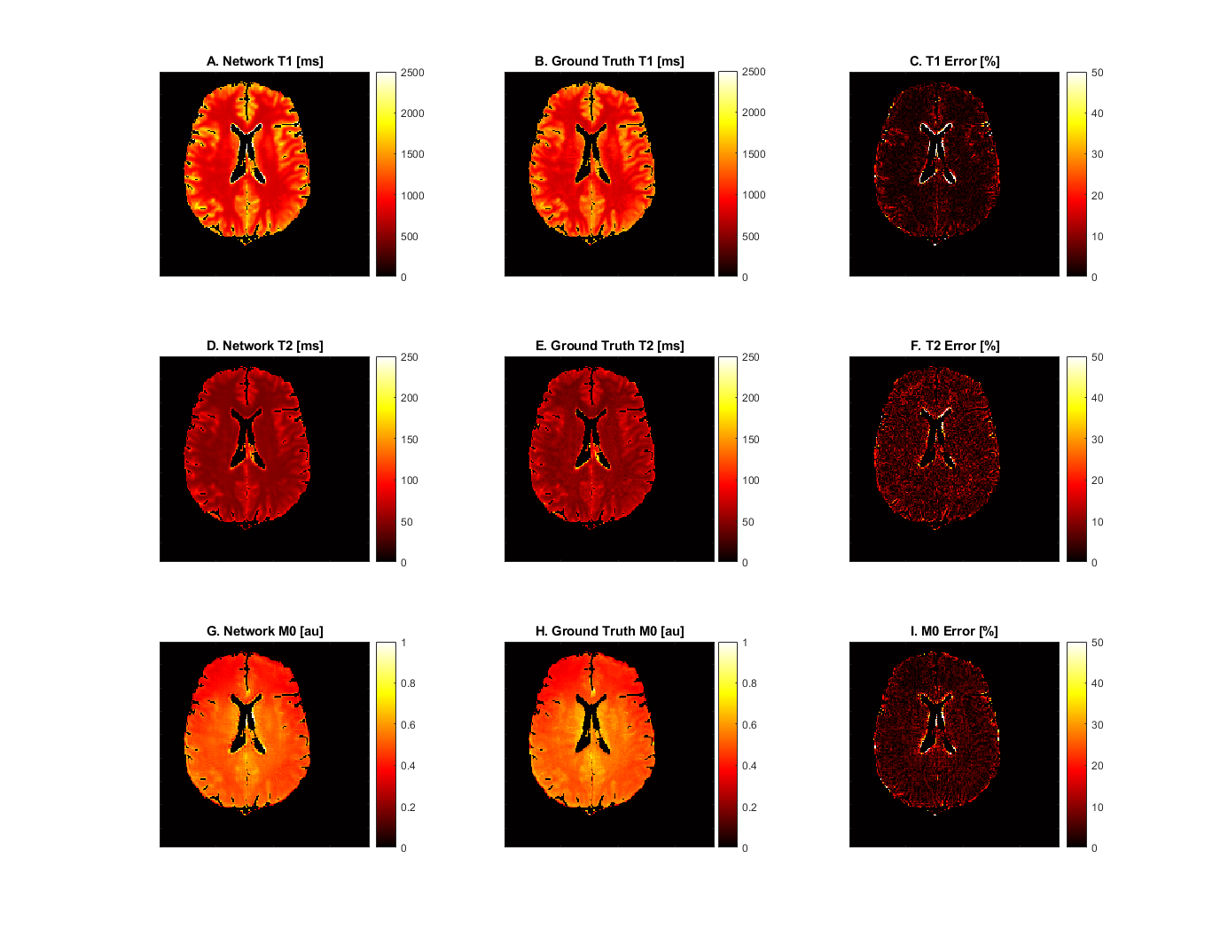
For the gray and white matter regions of the validation slices, the tissue parameters estimated by the network were compared against the ground truth tissue parameter maps used to simulate the dataset. The results of an example slice are depicted in figure 2. T1 values were predicted with an accuracy of 4.29 ± 13.9 percent, T2 values were predicted with an accuracy of 5.39 ± 5.42 percent, and M0 values were predicted with an accuracy of 4.81 ± 5.36 percent. Error in CSF regions were considerably higher.

Discussion

The self-supervised model performed well for T2 and M0 in the tissues of interest. Mean T1 error is also quite good, though its large standard deviation demands attention. Long T1 and T2 values of cerebro-spinal fluid (CSF) lead to the Bloch simulation having poor signal differentiation on the 4,800ms timescale over which the signal was simulated. We exclude CSF pixels as described in Results to focus on gray and white matter. Some partial volume pixels of CSF remain, especially around the central ventricle, leading to large errors in isolated locations on the validation slices. Outside these anomalies, T1 error is comparable to the T2 and M0 error.

Conclusion

We propose a physics-informed, self-supervised deep learning model for simultaneous quantification of three tissue properties from the MRF data without the need for ground truth tissue maps. The model performs well for all three tissue parameters of interest in grey- and white-matter areas, with an average of only 5% error as compared to the conventional dictionary matching results.

Acknowledgements

This work was supported in part by NIH grants R01 NS109439 and R21 EB026764.