3466
SMILR - Subspace MachIne Learning Reconstruction1Department of Electrical Engineering and Computer Science, Massachusetts Institute of Technology, Cambridge, MA, United States, 2Department of Radiology, Stanford University, Stanford, CA, United States, 3Department of Electrical Engineering, Stanford University, Stanford, CA, United States
Synopsis
Recent developments in spatiotemporal MRI techniques enable whole-brain multi-parametric mapping in incredibly short acquisition times through highly-efficient k-space encoding, subspace reconstruction and carefully-designed regularization. However, this comes at the cost of long reconstruction times making such methods difficult to integrate into clinical practice.
This abstract proposes a framework denoted SMILR (pronounced smile-r) to reduce the reconstruction times of subspace methods from multiple hours to a few minutes through machine learning. To evaluate performance, the framework is applied to multi-axis spiral projection MRF (denoted SPI-MRF) where it achieves improved reconstruction over conventional subspace reconstruction with locally low-rank at ~16-20x faster speed.
Introduction
Recent developments in spatiotemporal MRI techniques have enabled whole-brain multi-parametric mapping in incredibly short acquisition times[1,2,3]. These techniques leverage highly-efficient k-space encoding with subspace reconstruction[4] and carefully-designed regularization to achieve high-quality reconstruction without detrimental noise/artifact penalty despite high rates of acceleration. However, this comes at the cost of long reconstruction times for high-isotropic resolution volumetric imaging cases, making such methods difficult to integrate into clinical practice.This abstract proposes a framework denoted SMILR (pronounced smile-r) to reduce the reconstruction times of subspace methods from multiple hours to a few minutes through machine learning. To evaluate performance, the framework is applied to multi-axis spiral projection MRF (denoted SPI-MRF)[2] where it achieves improved reconstruction over conventional subspace reconstruction with locally low-rank at ~16-20x faster speed.
Design Considerations
Below are SMILR's steps for fast reconstruction of large volumetric spatiotemporal acquisition, along with their respective carefully-considered factors to reduce GPU-memory requirements.1. Leveraging MRI physics.
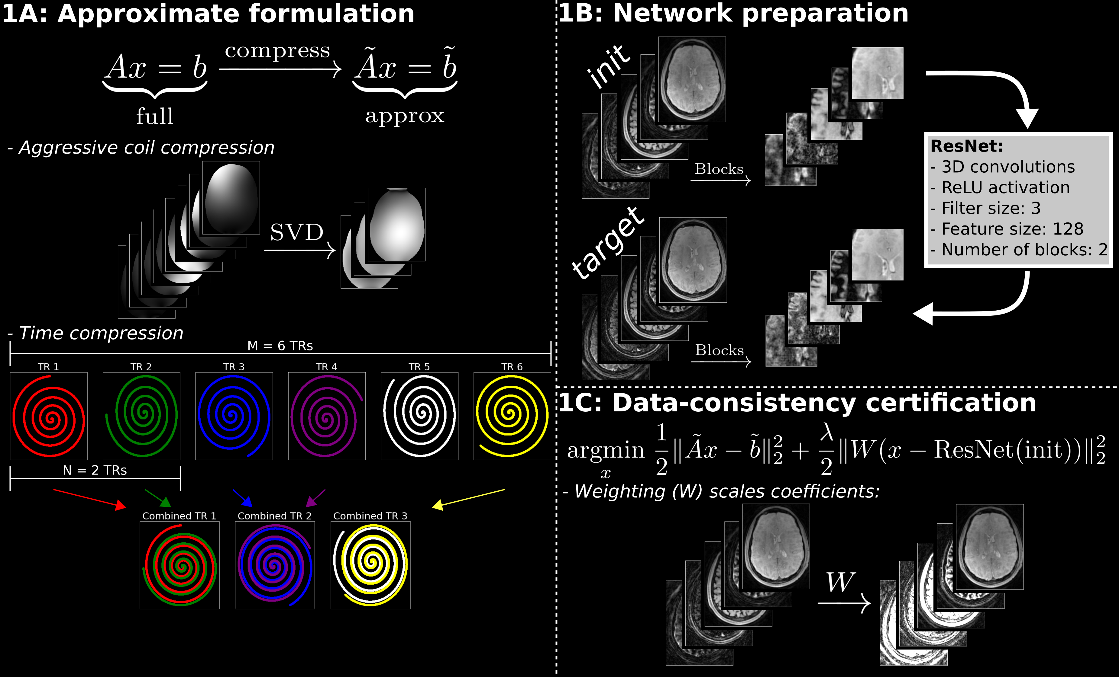
As a first step, in order to utilize prior coil sensitivity and the subspace basis information, an approximate reconstruction problem is formulated by performing aggressive SVD coil compression and reducing the TR dimension by combining adjacent N spirals in SPI-MRF as depicted in Figure 1A. This results in a small reconstruction problem with a reduced number of non-uniform Fourier transforms that easily fits into a GPU, enabling an ultra-fast approximate reconstruction that utilizes prior information from MRI physics. The resulting approximate reconstruction will be denoted as init.
2. High memory efficiency.
A subspace reconstruction yields multiple coefficient images, where each coefficient image is a large 3D-volume in SPI-MRF[2]. This prohibits the use of current unrolled machine-learning[5,6,7,8] methods due to extremely large memory requirements and/or very time-consuming data-consistency evaluations. In contrast, this work trains a network from and to blocks extracted from init and target (i.e., high quality 4-5 hour reconstructions), resulting in minimal memory use. This is depicted in Figure 1B. The trained network is then applied to init to obtain smilr.
3. Data consistency certification.
While the above allows for memory-efficient training, there is a risk of over-fitting as data-consistency is no longer integrated into the network. To enable robust use of machine learning, this work uses the inferred image as bias in a weighted least squares (WLS) reconstruction (see Figure 1C). This is similar to MoDL[5], except in this work, the network inference is used exactly once. Additionally, the WLS reconstruction is performed on the approximate problem used to generate init to enable fast processing of the entire pipeline. The end-result is denoted refine.
Note that SMILR enables machine-learning to be used on spatiotemporal acquisitions with full 3D-undersampling where data isn’t separable along readout within typical GPU-memory constraints.
Methods
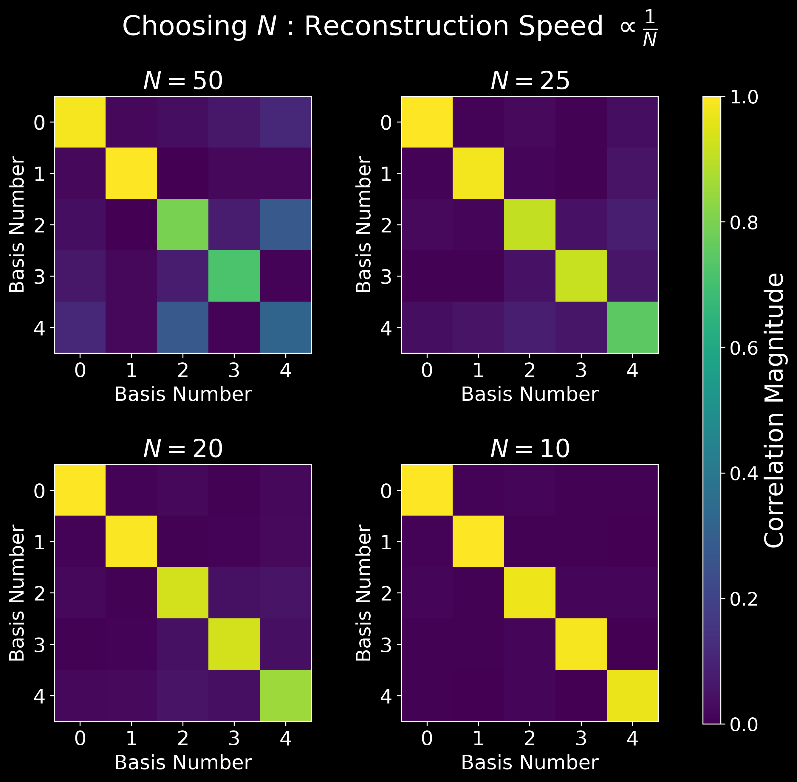
Data from nine healthy subjects were acquired on a 3T Premier MRI scanner (GE Healthcare, Waukesha, WI) and a 48-channel head receiver-coil using SPI-MRF[2] (M=500 TRs). The acquisition time was 6-minutes, acquired resolution was 1mm-iso, and FOV was 220mm-iso. The data were partitioned as 5 training/2 validation/2 testing and then retrospectively sub-sampled to simulate a 2-minute and 1-minute acquisition respectively. Coil sensitivity maps were estimated with JSENSE[9] from the simulated 1-minuted acquisition.All cases were reconstructed using conjugate gradient (CG) with BART[10] after SVD coil-compression to 10 coils to be used as reference. target denotes the 6-minute BART reconstruction. init was generated for all cases with N=25 and with coil compression to 3 coils using SigPy[11] with CG. N was determined as in Figure 2. All reconstructions were at 256mm-iso to avoid signal-wrap from the neck/shoulder. The Bloch Equation was used to generate a rank-5 subspace.
To prepare training data, for each training/validation subject, the following was repeated 24 times:
- Randomly select acceleration (6-minute, 2-minute or 1-minute acquisition).
- Randomly shift, flip and permute the volumetric (not coefficient) dimensions
- Partition result into blocks of shape$$$\;64\times64\times64\times5\;$$$(from$$$\;256\times256\times256\times5$$$), where 5 reflects the number of coefficients.
The refining step was performed using$$$\;W\;$$$(Figure 1C) with scaling values of [1,1,4,25,25] for coefficient images [1,2,3,4,5] respectively.
All BART reconstructions were performed with an Intel(R) Xeon(R) Gold 6138 CPU @ 2.00GHz with 376 GB of memory and 955 GB of swap. The init and refine reconstructions and network training was performed on an NVIDIA(R) Quadro GV100 with 32 GB VRAM. smilr was generated on the CPU.
Results
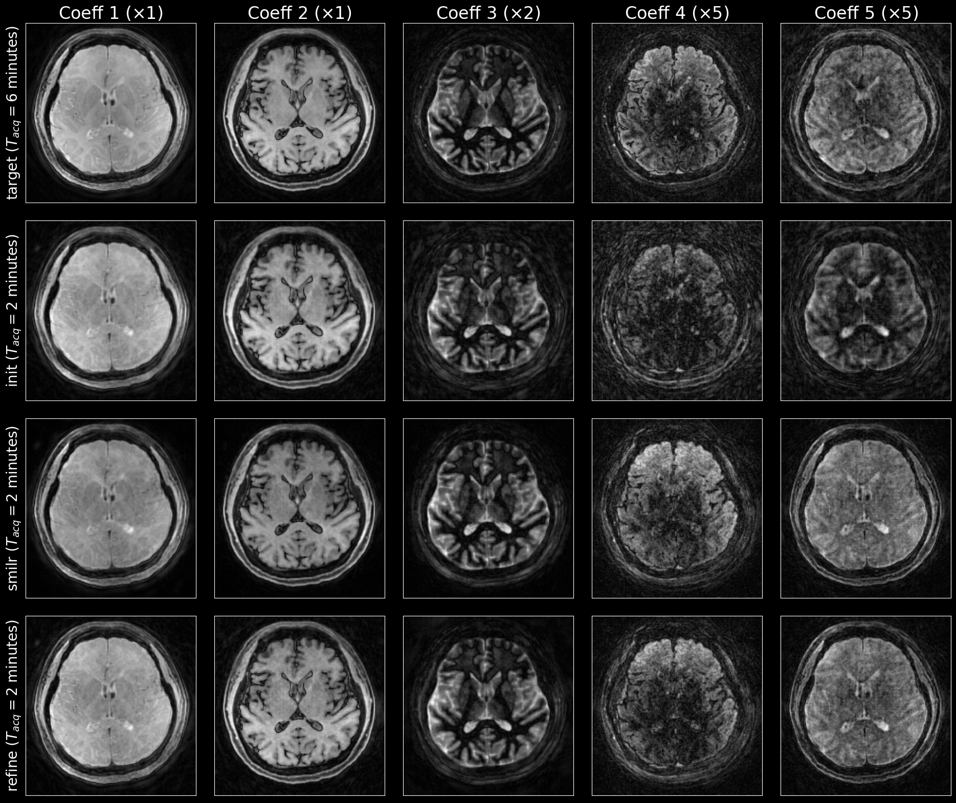
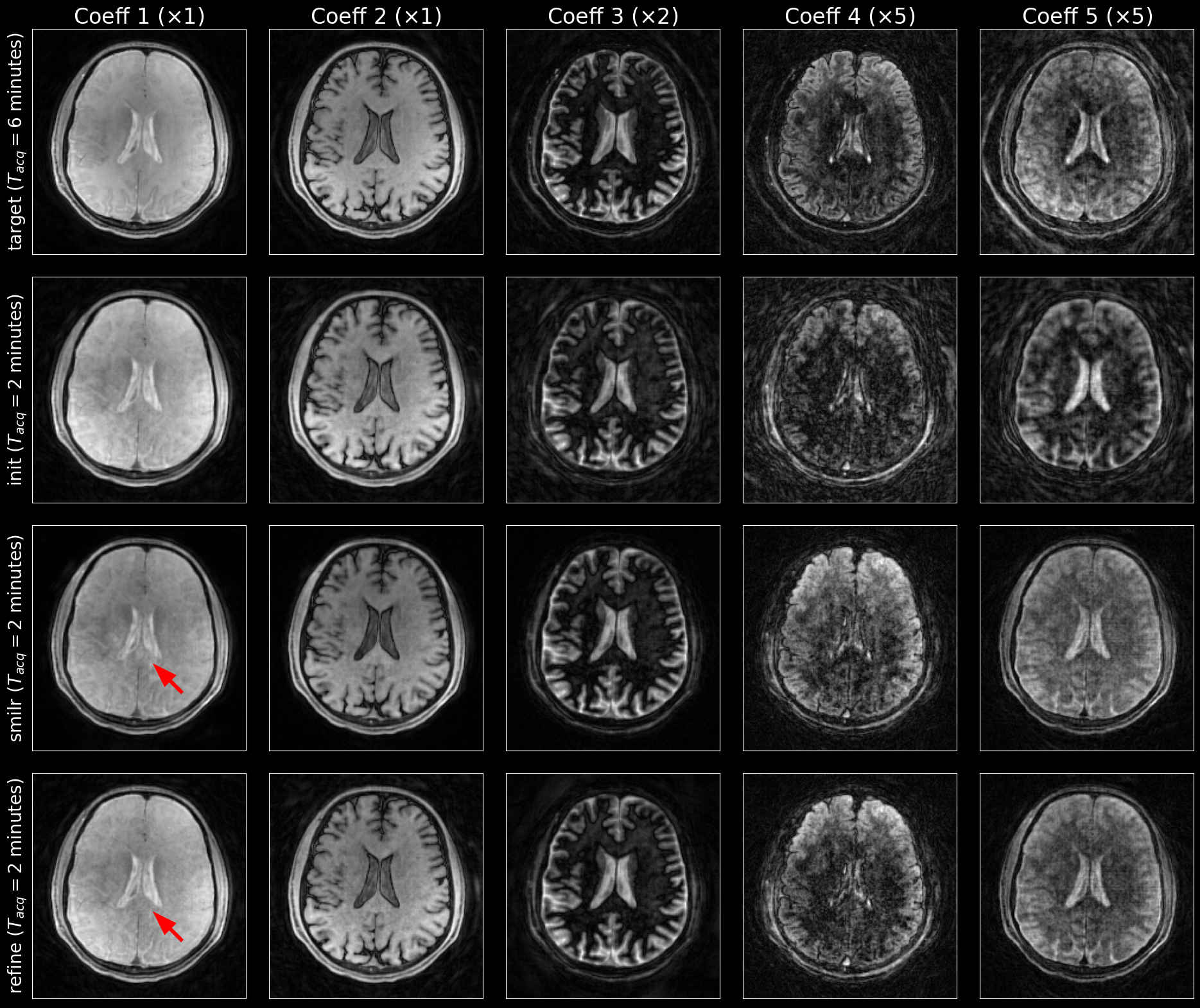
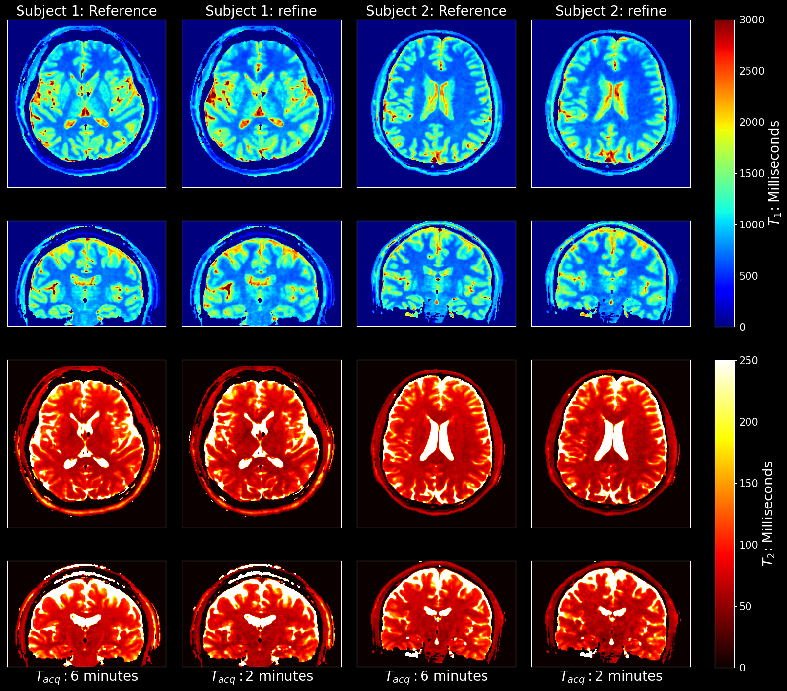
Figures 3 and 4 show the reconstruction results on the test subjects for the 2-minute acquisitions. The 1-minute acquisition requires additional parameter tuning, and will be future work. Figure 5 shows the resulting parametric maps and the respective reconstruction times. The entire SMILR pipeline took <15 minutes in contrast to ~4-5 hours required by the subspace reconstructions with locally low-rank.Discussion and Future Work
The SMILR framework enabled ~15 minute subspace reconstruction of spiral-MRF compared to 4-5 hours. WLS was used instead of a regular Tikhonov penalty (akin to MoDL) to account for ill-conditioning.Future work is to improve target by using subspace reconstruction with locally low-rank along with ESPIRiT[14] with SURE-based FOV-masking[15] to improve noise performance, incorporate ROVir[16] to kill shoulder/neck signal for more efficient coil compression and tune hyper-parameters for 1-minute SPI-MRF.
Acknowledgements
This study is supported in part by GE Healthcare research funds and NIHnR01EB020613, R01MH116173, R01EB019437, U01EB025162 , P41EB030006.References
- Wang, Fuyixue, et al. "Echo planar time‐resolved imaging (EPTI)." Magnetic resonance in medicine 81.6 (2019): 3599-3615.
- Cao, Xiaozhi, et al. "Optimized multi-axis spiral projection MR fingerprinting with subspace reconstruction for rapid whole-brain high-isotropic-resolution quantitative imaging." arXiv preprint arXiv:2108.05985 (2021).
- Christodoulou, Anthony G., et al. "Magnetic resonance multitasking for motion-resolved quantitative cardiovascular imaging." Nature biomedical engineering 2.4 (2018): 215-226.
- Liang, Zhi-Pei. "Spatiotemporal imagingwith partially separable functions." 2007 4th IEEE international symposium on biomedical imaging: from nano to macro. IEEE, 2007.
- Aggarwal, Hemant K., Merry P. Mani, and Mathews Jacob. "MoDL: Model-based deep learning architecture for inverse problems." IEEE transactions on medical imaging 38.2 (2018): 394-405.
- Sandino, Christopher M., et al. "Accelerating cardiac cine MRI using a deep learning‐based ESPIRiT reconstruction." Magnetic Resonance in Medicine 85.1 (2021): 152-167.
- Kellman, Michael, et al. "Memory-efficient learning for large-scale computational imaging." IEEE Transactions on Computational Imaging 6 (2020): 1403-1414.
- Hammernik, Kerstin, et al. "Learning a variational network for reconstruction of accelerated MRI data." Magnetic resonance in medicine 79.6 (2018): 3055-3071.
- Ying, Leslie, and Jinhua Sheng. "Joint image reconstruction and sensitivity estimation in SENSE (JSENSE)." Magnetic Resonance in Medicine: An Official Journal of the International Society for Magnetic Resonance in Medicine 57.6 (2007): 1196-1202.
- Uecker, Martin, et al. "Berkeley advanced reconstruction toolbox." Proc. Intl. Soc. Mag. Reson. Med. Vol. 23. No. 2486. 2015.
- Ong, Frank, and Michael Lustig. "SigPy: a python package for high performance iterative reconstruction." Proceedings of the International Society of Magnetic Resonance in Medicine, Montréal, QC 4819 (2019).
- He, Kaiming, et al. "Deep residual learning for image recognition." Proceedings of the IEEE conference on computer vision and pattern recognition. 2016.
- Falcon, William, and Kyunghyun Cho. "A framework for contrastive self-supervised learning and designing a new approach." arXiv preprint arXiv:2009.00104 (2020).
- Uecker, Martin, et al. "ESPIRiT—an eigenvalue approach to autocalibrating parallel MRI: where SENSE meets GRAPPA." Magnetic resonance in medicine 71.3 (2014): 990-1001.
- Iyer, Siddharth, et al. "SURE‐based automatic parameter selection for ESPIRiT calibration." Magnetic Resonance in Medicine 84.6 (2020): 3423-3437.
- Kim, Daeun, et al. "Region‐optimized virtual (ROVir) coils: Localization and/or suppression of spatial regions using sensor‐domain beamforming." Magnetic Resonance in Medicine 86.1 (2021): 197-212.
Figures