3458
Deep generative model for learning tractography streamline embeddings based on a Convolutional Variational Autoencoder1Imaging Genetics Center, Mark and Mary Stevens Neuroimaging and Informatics Institute, Keck School of Medicine, University of Southern California, Marina Del Rey, CA, United States, 2Department of Intelligent Systems Engineering, School of Informatics, Computing, and Engineering, Indiana University Bloomington, Bloomington, IN, United States
Synopsis
We present a deep generative model to autoencode tractography streamlines into a smooth low dimensional latent distribution, which captures their spatial and sequential information with 1D convolutional layers. Using linear interpolation, we show that the learned latent space translates smoothly into the streamline space and can decode meaningful outputs from sampled points. This allows for inference on new data and direct use of Euclidean distance on the embeddings for downstream tasks, such as bundle labeling, quantitative inter-subject comparisons, and group statistics.
Introduction
Streamlines extracted from whole-brain fiber tractography are often used to study white matter fiber pathways and brain structural connectivity. Processing such streamlines is computationally intensive given the large amount of data, and methods based on nonlinear dimensionality reduction1 and autoencoders (AE)2,3,4 have been proposed to learn streamlines embeddings to enable efficient downstream analysis, such as filtering and bundle labeling.However, AEs trained with only reconstruction loss can easily overfit to training data, and not every point in the embedding space is meaningful. In this work, we use variational AE (VAE)5 with 1D convolution (ConvVAE) to learn a generative model that learns a smooth latent distribution of streamlines; we validate the learned embeddings using interpolation and K-nearest neighbor (KNN) methods.
Methods
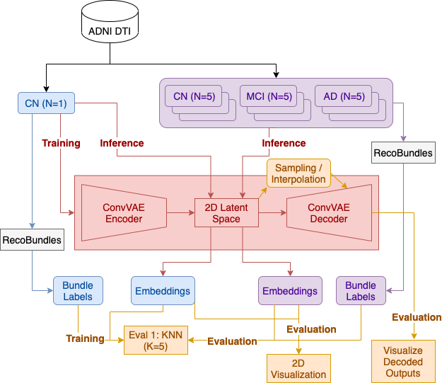
We analyzed multi-shell diffusion MRI data from 141 subjects (age: 55-91 years, 80F, 61M) - 87 cognitively normal controls (CN), 44 with mild cognitive impairment (MCI), 10 with dementia (AD) - from the Alzheimer’s Disease Neuroimaging Initiative (ADNI) database6. dMRI were preprocessed with the ADNI3 dMRI protocol, correcting for noise7,8,9,10, Gibbs ringing11, eddy currents12,13,14, bias field inhomogeneity and echo planar imaging distortion artifacts.We applied multishell constrained spherical deconvolution (CSD) to reconstruct orientation distribution functions (ODF) and applied a probabilistic particle filtering tracking algorithm to generate whole-brain tractograms from the preprocessed dMRI. 30 white matter tracts per subject were extracted using auto-calibrated DIPY’s7 RecoBundles15. Selecting one control subject (with 51,654 streamlines from 30 bundles) for training and five subjects from each diagnostic group (CN/MCI/AD) for inference, we further preprocessed streamlines into 256 3D points per curve, standardized to have zero mean and identity covariance.
The ConvVAE encoder consists of three convolutional layers with kernel sizes 256, 128 and 64 and a symmetric decoder, with a total of 1.6m parameters. The large kernel sizes allow the model to learn sequential information from streamlines. The model was trained with Evidence lower bound (ELBO) loss with Gaussian likelihood instead of pixel-wise MSE as the reconstruction term, and Kullback–Leibler divergence as the regularization term. The embedding dimension was set to 2 to allow for direct visualization.
We first evaluated the model by visualizing 2D embeddings and reconstructed streamlines. To then evaluate the generative process, we sampled linearly interpolated points from the latent space and visualized the decoded streamlines. The minimum average direct-flip (MDF) distance16 was calculated between consecutive interpolated streamlines to validate if the decoder learned a smooth manifold in the streamline space2. We further used KNN with L2 distance to calculate the agreement between the embeddings and given labels. The model training, inference and evaluation steps are shown in Figure 1.
Results
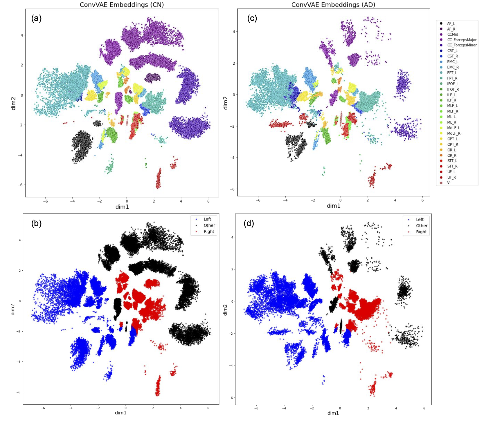
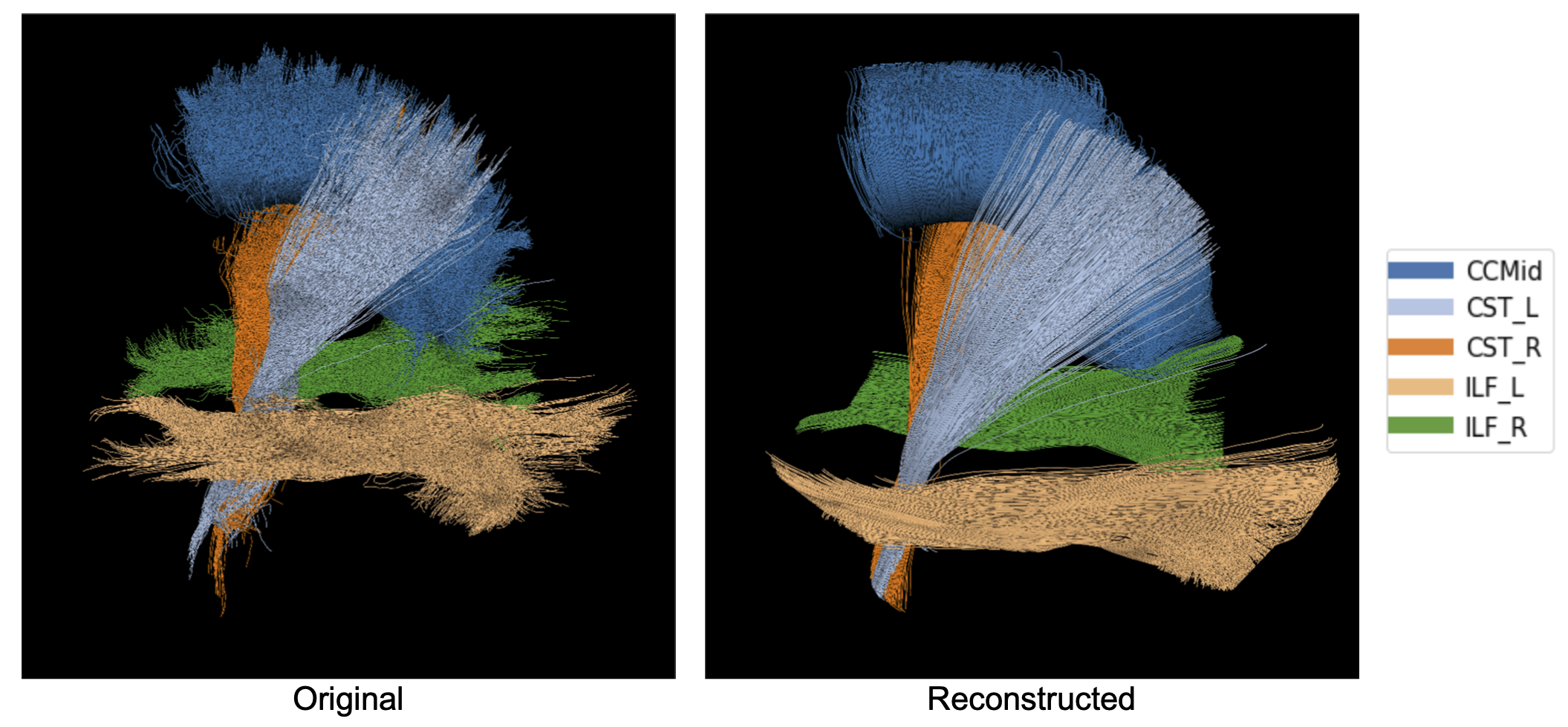
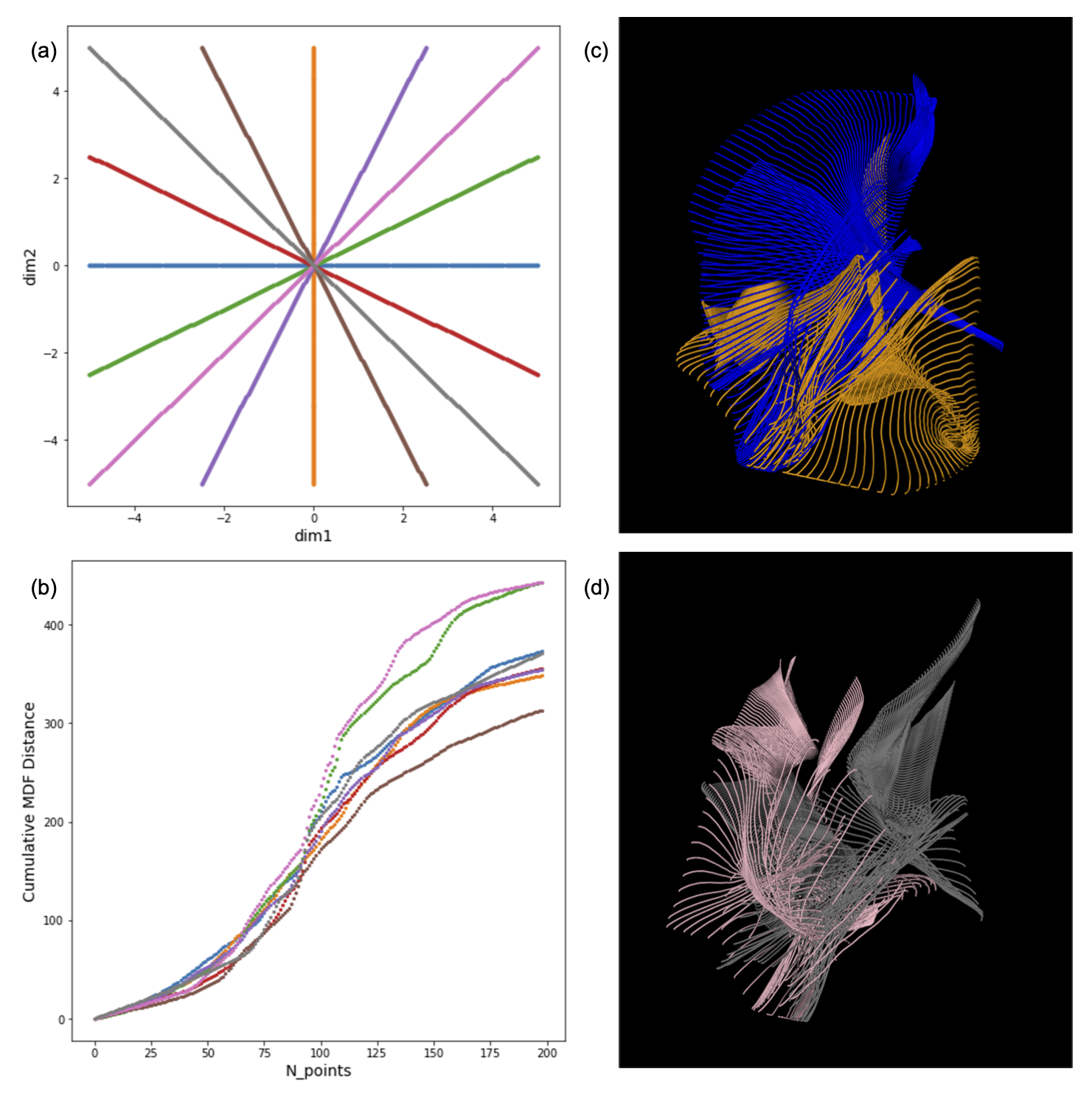
Figure 2a-2b depicts the 2D embeddings of the trained subject data, labeled by bundles and hemispheres, respectively. Corresponding bundles from the left and right hemispheres fall into distinct clusters in the latent space. Overlapping bundles in the latent space also overlap in the streamline space, where endpoints are in close proximity and streamlines follow similar trajectories. Reconstructed streamlines (Figure 3) retain the global structure of streamlines, but are smoother; more detail may be preserved with a higher dimensional latent space.Eight linear interpolations (each with 200 points at different orientations in the latent space) were decoded to generate new streamlines (Figure 4a). Cumulative MDF distances starting from one end to the other for each interpolation are plotted in Figure 4b. We see that the distances follow a sigmoidal curve, where those for points near (0,0) in the latent space follow a linear trajectory, and embedded points farther from (0,0) are closer to each other in the streamline space. Two sets of generated streamlines from orthogonal interpolations are plotted in Figure 4c-4d.
Since many embedding points are centered at 0 (Figure 2a), we apply Euclidean distances to the latent space. We validate that this mapping applies to new data by encoding streamlines from 15 subjects during inference, and found that their embeddings fall near the trained embeddings for corresponding bundles (see Figure 2c-2d for embeddings of a randomly selected AD subject). Fitting a KNN model on embeddings from the subject used to train the ConvVAE, the weighted average accuracy for each group is 80.4% (CN), 78.9% (MCI) and 74.6% (AD).
Discussion
With latent dimension of 2, visualizations show that our generative ConvVAE model can learn low-dimensional embeddings with distinct clusters for defined bundles that can be used to compare those learned from different subjects. Interpolation results show that the learned manifold is smooth, but there exist variations at different locations in latent space, shown by the varying slopes in Figure 4b. This could be due to overfitting on single subject data or streamline imbalance in different bundles. In future work, we plan to explore training on multi-subject data, with higher latent space dimension, to learn subject-invariant features and a more robust latent space.Conclusion
Here, we present a deep generative model using a ConvVAE. The model learns a smooth latent distribution of inputs from tractography streamlines which captures their spatial information, allows sampling and yields meaningful decoded outputs. We show that the 2D latent space translates smoothly into the streamline space, allowing us to use Euclidean distance for downstream tasks such as bundle labeling and quantitative inter-subject comparisons.Acknowledgements
This work was supported by the NIH (National Institutes of Health) under the AI4AD project grant U01 AG068057, grant numbers P41 EB015922, and RF1AG057892.References
[1] B. Q. Chandio et al., “FiberNeat: unsupervised streamline clustering and white matter tract filtering in latent space,” bioRxiv 2021. doi: 10.1101/2021.10.26.465991.
[2] J. H. Legarreta et al., “Filtering in tractography using autoencoders (FINTA),” Medical Image Analysis, vol. 72, p. 102126, Aug. 2021, doi: 10.1016/j.media.2021.102126.
[3] S. Zhong, Z. Chen, and G. Egan, “Auto-encoded Latent Representations of White Matter Streamlines for Quantitative Distance Analysis,” bioRxiv 2021. doi: 10.1101/2021.10.06.463445.
[4] M. Chamberland et al., “Tractometry-based Anomaly Detection for Single-subject White Matter Analysis,” arXiv:2005.11082 [cs, q-bio], May 2020, Accessed: Nov. 08, 2021. [Online]. Available: http://arxiv.org/abs/2005.11082
[5] D. P. Kingma and M. Welling, “Auto-Encoding Variational Bayes,” arXiv:1312.6114 [cs, stat], May 2014, Accessed: Oct. 08, 2021. [Online]. Available: http://arxiv.org/abs/1312.6114
[6] A. Zavaliangos-Petropulu et al., “Diffusion MRI Indices and Their Relation to Cognitive Impairment in Brain Aging: The Updated Multi-protocol Approach in ADNI3,” Front. Neuroinform., vol. 13, p. 2, Feb. 2019, doi: 10.3389/fninf.2019.00002.
[7] E. Garyfallidis et al., “Dipy, a library for the analysis of diffusion MRI data,” Front. Neuroinform., vol. 8, Feb. 2014, doi: 10.3389/fninf.2014.00008.
[8] J. V. Manjón, P. Coupé, L. Concha, A. Buades, D. L. Collins, and M. Robles, “Diffusion Weighted Image Denoising Using Overcomplete Local PCA,” PLoS ONE, vol. 8, no. 9, p. e73021, Sep. 2013, doi: 10.1371/journal.pone.0073021.
[9] J. Veraart, E. Fieremans, and D. S. Novikov, “Diffusion MRI noise mapping using random matrix theory: Diffusion MRI Noise Mapping,” Magn. Reson. Med., vol. 76, no. 5, pp. 1582–1593, Nov. 2016, doi: 10.1002/mrm.26059.
[10] J. Veraart, D. S. Novikov, D. Christiaens, B. Ades-aron, J. Sijbers, and E. Fieremans, “Denoising of diffusion MRI using random matrix theory,” NeuroImage, vol. 142, pp. 394–406, Nov. 2016, doi: 10.1016/j.neuroimage.2016.08.016.
[11] E. Kellner, B. Dhital, V. G. Kiselev, and M. Reisert, “Gibbs-ringing artifact removal based on local subvoxel-shifts: Gibbs-Ringing Artifact Removal,” Magn. Reson. Med., vol. 76, no. 5, pp. 1574–1581, Nov. 2016, doi: 10.1002/mrm.26054.
[12] J. L. R. Andersson and S. N. Sotiropoulos, “An integrated approach to correction for off-resonance effects and subject movement in diffusion MR imaging,” NeuroImage, vol. 125, pp. 1063–1078, Jan. 2016, doi: 10.1016/j.neuroimage.2015.10.019.
[13] J. L. R. Andersson, M. S. Graham, E. Zsoldos, and S. N. Sotiropoulos, “Incorporating outlier detection and replacement into a non-parametric framework for movement and distortion correction of diffusion MR images,” NeuroImage, vol. 141, pp. 556–572, Nov. 2016, doi: 10.1016/j.neuroimage.2016.06.058.
[14] J. L. R. Andersson, M. S. Graham, I. Drobnjak, H. Zhang, N. Filippini, and M. Bastiani, “Towards a comprehensive framework for movement and distortion correction of diffusion MR images: Within volume movement,” NeuroImage, vol. 152, pp. 450–466, May 2017, doi: 10.1016/j.neuroimage.2017.02.085.
[15] B. Q. Chandio et al., “Bundle analytics, a computational framework for investigating the shapes and profiles of brain pathways across populations,” Sci Rep, vol. 10, no. 1, p. 17149, Dec. 2020, doi: 10.1038/s41598-020-74054-4.
[16] E. Garyfallidis, M. Brett, M. M. Correia, G. B. Williams, and I. Nimmo-Smith, “QuickBundles, a Method for Tractography Simplification,” Front Neurosci, vol. 6, p. 175, 2012, doi: 10.3389/fnins.2012.00175.
Figures