Motivation

Sensitivity Encoding (SENSE) is an established parallel imaging method [1], and admits regularization terms that can lead to better reconstruction. For example, L2-SENSE algorithm adds an L2 (i.e. Tikhonov) penalty on the image [2], while L1-SENSE combines SENSE with compressed sensing (CS) to penalize the L1 norm in a sparsifying domain (e.g. Wavelets) [3, 4]. Despite their effectiveness, these regularized algorithms have certain limitations. They often require effort in tuning a regularization penalty, which may be difficult to identify without knowledge of the ground-truth image. In addition, they do not quantify model uncertainty, which can indicate where reconstruction errors are likely to occur.

Method

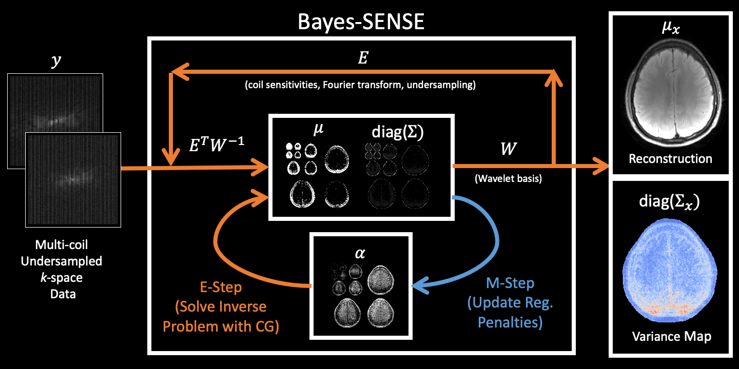
Bayes-SENSE reconstructs an image $$$x\in\mathbb{C}^N$$$ from undersampled k-space measurements $$$y\in\mathbb{C}^{N \cdot C / R}$$$, where $$$R$$$ is the undersampling factor and $$$C$$$ is the number of coils. Fig1 provides a diagram of the reconstruction.

Model: The basic SENSE model assumes that $$$y = Ex+\varepsilon$$$, where $$$\varepsilon$$$ is k-space noise and $$$E\in\mathbb{C}^{N\cdot C/R\times N}$$$ is the encoding matrix containing the sensitivity coils, Fourier transform, and undersampling masks. In Bayes-SENSE, we extend this model by combining it with BCS [5]. We assume that $$$x=Wz$$$, where $$$W\in\mathbb{C}^{N \times N}$$$ is an orthogonal transform (e.g. Wavelet basis) and $$$z\in\mathbb{C}^N$$$ is a vector of sparse coefficients. Let $$$\alpha\in\mathbb{R}^N$$$ be a vector of regularization penalties for each element of $$$z$$$. We impose a $$$\mathcal{N}(0, 1/\alpha_i)$$$ prior on each pair $$$(\text{Real}(z_i), \text{Imag}(z_i))$$$. Then, the k-space data is modeled as $$$y=\Phi z + \varepsilon$$$, where $$$\Phi=EW$$$.


Inference: We perform inference on this model using the Expectation-Maximization (EM) algorithm. We iteratively alternate between an E-Step, which solves for a posterior distribution $$$p(z|y)=\mathcal{N}(\mu, \Sigma)$$$, and an M-Step, which updates the regularization penalties $$$\alpha$$$: $$\mu=\beta\Sigma \Phi^\top y, \quad\Sigma=\left(\beta\Phi^\top \Phi + \text{diag}(\alpha))\right)^{-1}\quad\text{(E-Step)}$$ $$\alpha_i=\frac{2}{\text{Real}(\mu_i)^2+\text{Real}(\Sigma_{i,i})+\text{Imag}(\mu_i)^2+\text{Imag}(\Sigma_{i,i})} \forall i=1,2,\ldots,N\quad\text{(M-Step)}$$ For images with a large number of pixels $$$N$$$, directly applying these EM updates can be very expensive due to the matrix inversion needed by the E-Step. To resolve this issue, we follow [6, 7] in using the conjugate gradient (CG) algorithm to directly solve for $$$\mu$$$ and probe the diagonal elements of $$$\Sigma$$$ without needing to compute $$$\Sigma$$$ itself. Thus, the time complexity of Bayes-SENSE inference scales as $$$O(N\log N)$$$, which is asymptotically the same as L2-SENSE/L1-SENSE.

Image Reconstruction and Variance Map: After running EM for $$$T$$$ iterations, we can recover a posterior distribution for the image as $$$x|y\sim\mathcal{N}(\mu_x,\Sigma_x)$$$, where $$$\mu_x=W\mu$$$ and $$$\Sigma_x=W\Sigma W^\top$$$. The mode of this distribution $$$\mu_x$$$ is our reconstructed image and the diagonal elements of $$$\Sigma_x$$$ form a pixel-wise variance map.

Unlike L2-SENSE and L1-SENSE, Bayes-SENSE does not require tuning of regularization penalties because its penalties $$$\alpha$$$ are learned from the data. Like BCS [5, 6], Bayes-SENSE is easy to extend to multi-contrast reconstruction by having all contrasts share a common $$$\alpha$$$ vector of regularization penalties. We call this extension Joint Bayes-SENSE, which can efficiently parallelize the multi-contrast E-Steps across multi-core machines.

Experiments

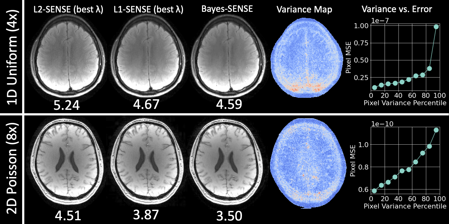
We compare L2-SENSE, L1-SENSE, and Bayes-SENSE on several reconstruction tasks. In all cases, we report best results after tuning the regularization penalty $$$\lambda$$$ for L2-SENSE and for L1-SENSE. For L1-SENSE and Bayes-SENSE, we use 3-level Daubechies-2 wavelets. We run Bayes-SENSE for $$$T=8$$$ iterations with $$$K=10$$$ CG probe vectors. All acquisitions are made with 32ch coils. Code/data can be found at https://anonymous.4open.science/r/bayes-sense-BF92/. We use the SigPy package [8] for L2-/L1-SENSE implementations.

Fig2. presents results for reconstruction of (1) a 256x256 in-vivo FLAIR image with uniform undersampling in 1D at $$$R=4$$$ and (2) a 224x210 in-vivo $$$T_2*$$$-weighted image with Poisson undersampling in 2D at $$$R=8$$$. In both cases, we show that Bayes-SENSE outperforms L2- and L1-SENSE in NRMSE, while not needing $$$\lambda$$$-tuning. Bayes-SENSE also generates variance maps that correlate well with reconstruction error.

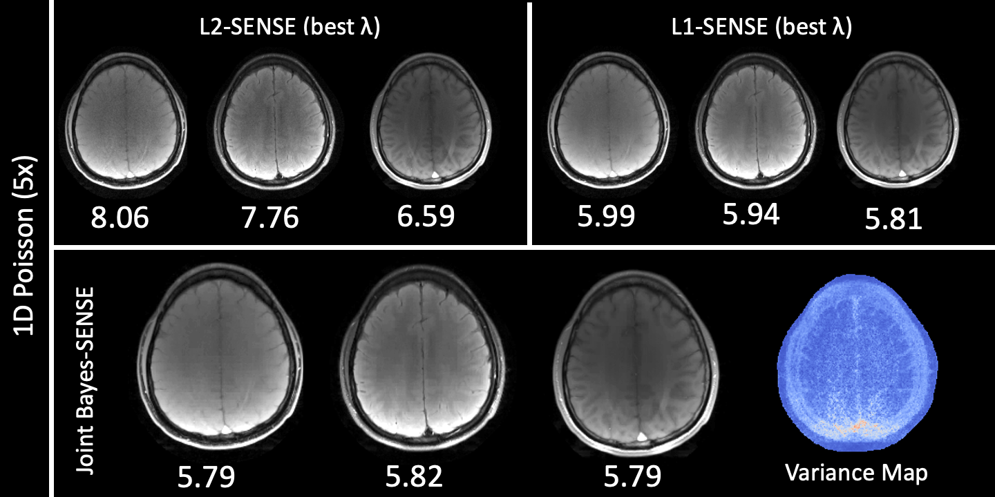
Fig3. presents results for reconstruction of three 256x256 in-vivo images (GRE, $$$T_2$$$-weighted, FLAIR) from $$$R=5$$$ uniform undersampling in 1D at $$$R=5$$$. Joint Bayes-SENSE outperforms L2-SENSE and slightly outperforms L1-SENSE in terms of NRMSE, while automatically tuning regularization penalties for all contrasts simultaneously.

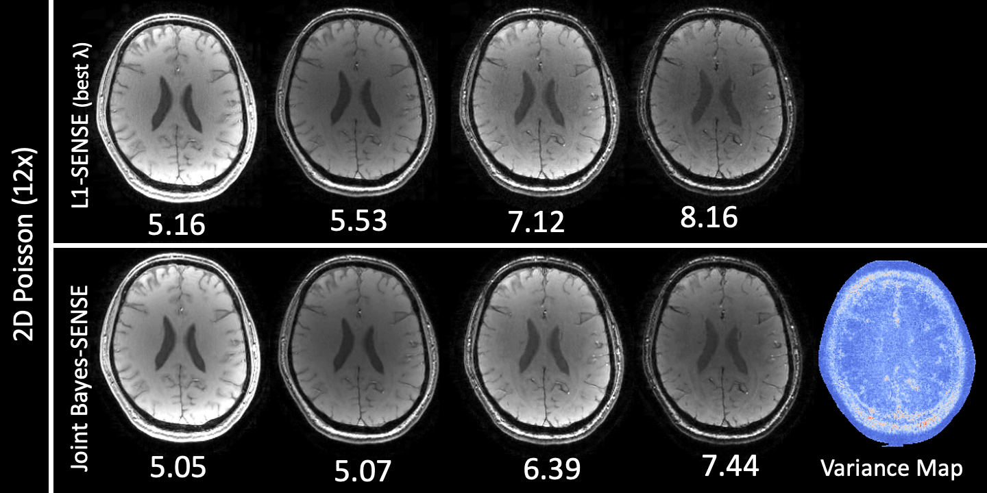
Fig4. presents results for reconstruction of four 224x210 in-vivo $$$T_2*$$$-weighted echoes with Poisson undersampling in 2D at $$$R=12$$$. Joint Bayes-SENSE outperforms both L2-SENSE (not pictured) and L1-SENSE in NRMSE on all contrasts by leveraging the shared information among the contrasts.

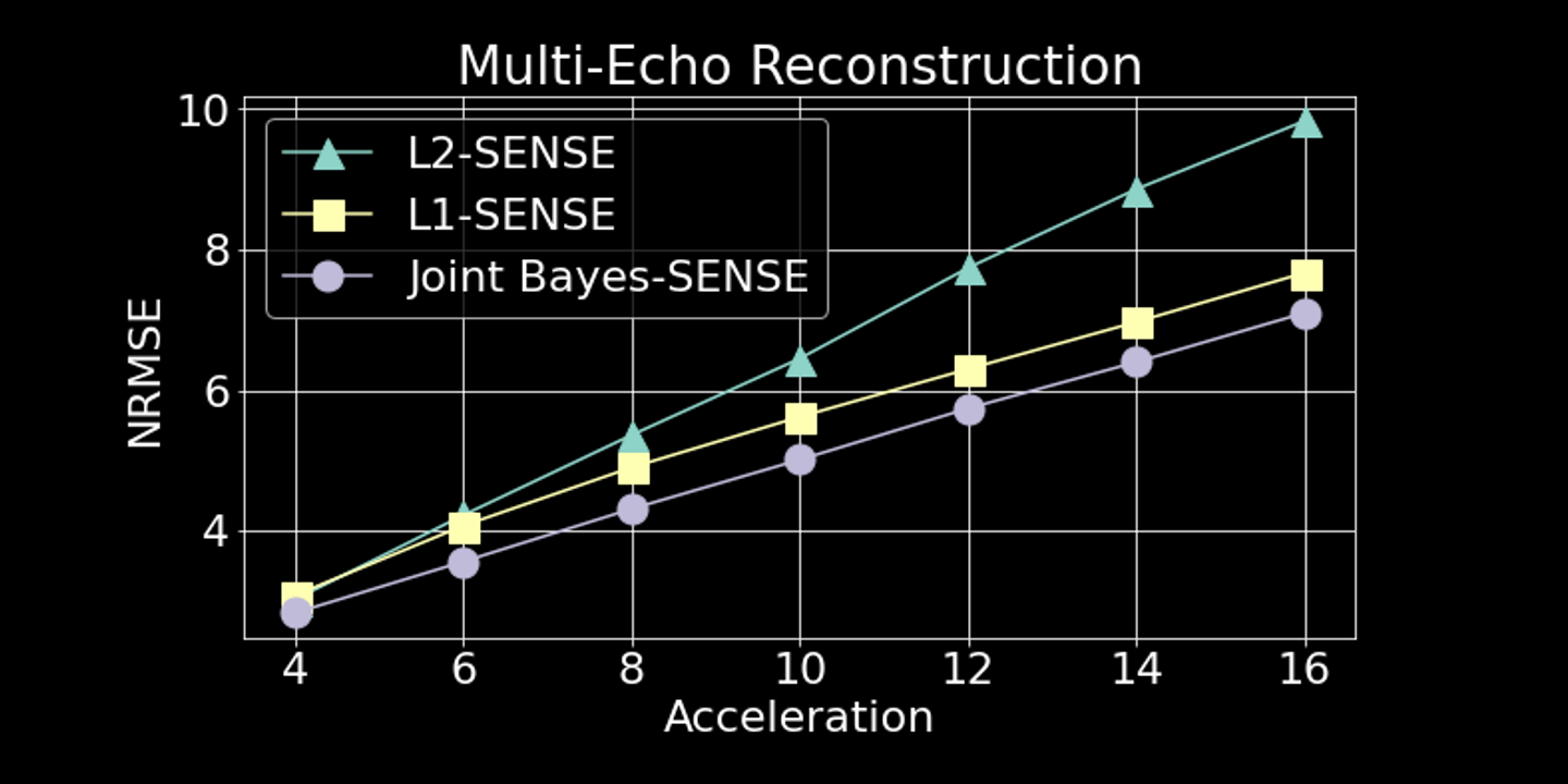
Fig5. We repeat the experiment in Fig4 for undersampling factors $$$R=4,6,8,10,12,14,16$$$. Joint Bayes-SENSE consistently outperforms L2-SENSE and L1-SENSE in terms of overall NRMSE. To process four contrasts, L2-SENSE/L1-SENSE take ~2-3 minutes on CPU while Bayes-SENSE takes ~3-4 minutes on GPU.

Discussion/Conclusion

In this work, we introduced Bayesian Sensitivity Encoding, which can improve upon L2-/L1-SENSE by providing automatic regularization tuning, uncertainty quantification, and the ability to integrate multi-contrast data for joint reconstruction. Future work will tackle further reducing the computational cost of Bayes-SENSE by exploiting preconditioning for CG. As the memory footprint of the reconstruction is small, several slices can be processed in parallel on GPU, thereby providing further speed-up.

Acknowledgements

This work was supported by research grants NIH R01 EB028797, R03 EB031175, U01 EB025162, P41 EB030006, U01 EB026996, and the NVidia Corporation and Amazon AWS Research Awards for computing support.