Introduction

Magnetic resonance T1 mapping brings enhanced tissue contrast, it is widely used to detect and monitor the progressions of epilepsy, Alzheimer's and Parkinson's diseases, etc. [1-3]. High-resolution volumetric imaging provides necessary information to detect small pathological changes in the tissue, but its long scan time causes discomfort to the patients, which increases the chance of patient motion and brings artifacts to images. Undersampling is thus adopted to reduce the scan time by acquiring data according to various undersampling patterns. Although the motion artifacts are greatly alleviated, image quality now suffers from missing data in the k-space. Sparse prior on the image wavelet coefficients is often used to fill in the missing information through a regularization term. The regularization parameter needs to be manually tuned to balance the tradeoff between data-fidelity and regularization. However, parameter tuning is not only time-consuming, but also becomes a problem for prospective sampling schemes where training data is unavailable. On the other hand, measurements of quantitative T1 and T2* using variable flip-angle multi-echo gradient echo (GRE) sequence pose additional challenges. The conventional approach is to compute T1 maps separately from individual echo and then average them. It does not take account of additional information from the underlying exponential decay model among multi-echo measurements, which is valuable in case of limited data due to undersampling. In order to address these two issues, here we propose a Bayesian approach that automatically estimates the parameters and incorporates the exponential decay model into its probabilistic inference.

Proposed Method

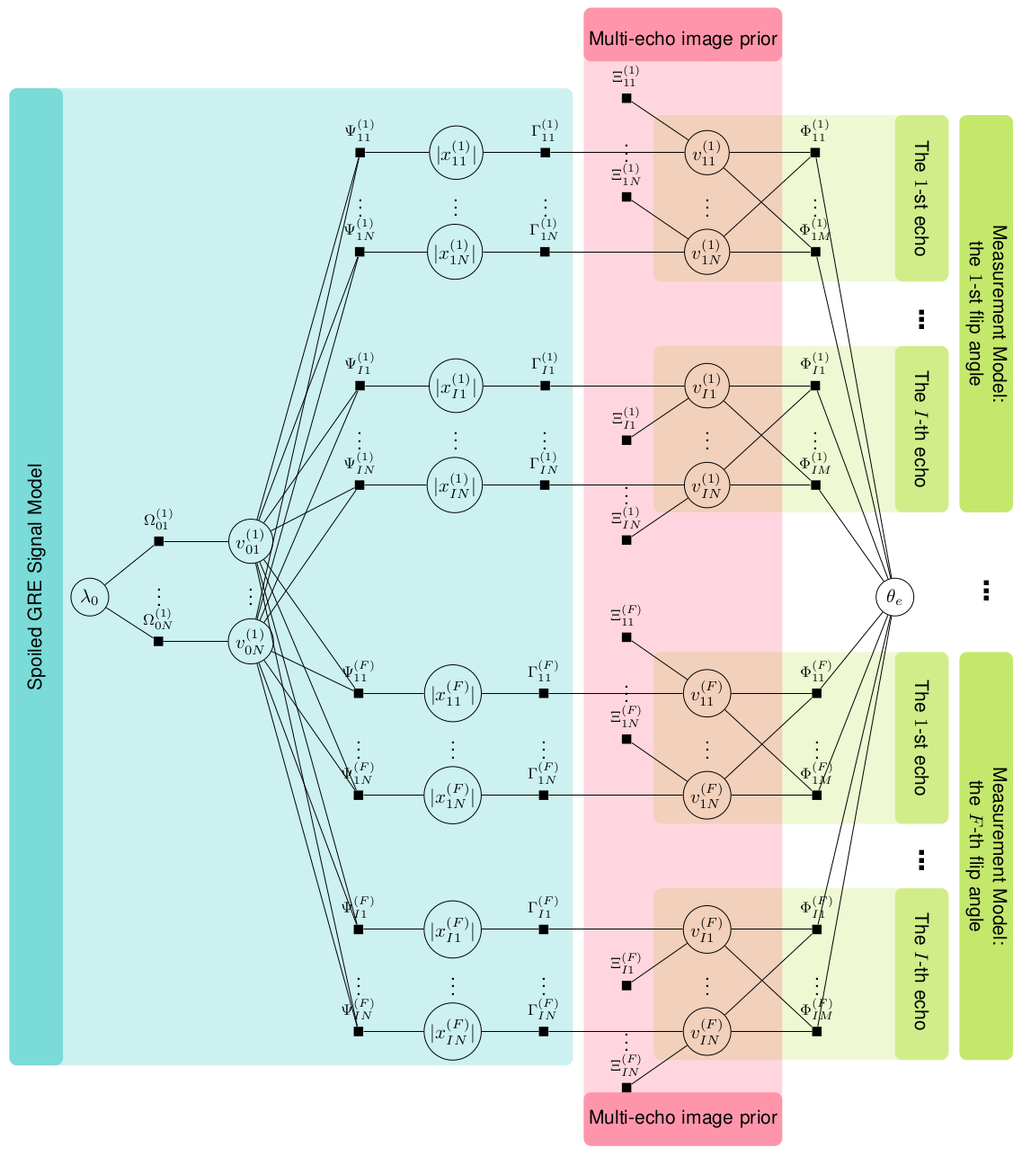
The wavelet coefficients $$$\boldsymbol v$$$ of an image $$$\boldsymbol x$$$ are assumed to be independent and identically distributed (i.i.d.) and follow a sparse prior distribution like Laplace: $$$p(v|\lambda)=\lambda\exp(-\lambda |v|)$$$, where $$$\lambda$$$ is the distribution parameter. The measurements are $$$\boldsymbol y=\boldsymbol A\boldsymbol v+\boldsymbol w$$$, where $$$\boldsymbol A$$$ is the measurement matrix, $$$\boldsymbol w$$$ contains i.i.d white Gaussian noise: $$$p(w|\theta)=\mathcal{N}(w|0,\theta)$$$, and $$$\theta$$$ is noise variance. We compute the maximum-a-posteriori estimation using approximate message passing (AMP) [4], i.e. $$$\hat{v}=\arg\max_v p(v|\boldsymbol y)$$$. The distribution parameters $$$\{\lambda,\theta\}$$$ are treated as random variables and jointly estimated with the coefficients $$$\boldsymbol v$$$ [5].

The standard AMP was developed for linear system, and could not be used to recover $$$T_1$$$ map in the nonlinear spoiled GRE signal model. We thus propose a new nonlinear AMP framework to resolve this issue, and its factor graph is shown in Fig. 1. Suppose that measurements are acquired at $$$I$$$ echo times for each of $$$F$$$ flip angles. There are three blocks in the factor graph:
1) The spoiled GRE signal model encodes the nonlinear relationship between the initial magnetization $$$\boldsymbol x_0$$$ and the signals $$$\{\boldsymbol x_i^{(f)}\}_{i,f}$$$ at multiple echo times $$$\{t_i\}_i$$$ and multiple flip angles $$$\{\alpha_f\}_f$$$:
$$|x_i^{(f)}|=x_0\cdot\sin(\alpha_f)\cdot\frac{1-e^{-TR/T_1}}{1-\cos\alpha_f\cdot e^{-TR/T_1}}\cdot e^{-t_i/T_2^*},$$
where $$$TR$$$ is the repetition time, $$$T_1$$$ is the T1 relaxation time, $$$T_2^*$$$ is the T2* relaxation time. With $$$|x_i^{(f)}|$$$ and $$$x_0$$$ fixed, $$$T_1$$$ and $$$T_2^*$$$ can be computed as the least square solutions to the above signal model.
2) The multi-echo image prior encodes the sparse prior on the image wavelet coefficients $$$\{\boldsymbol v_i^{(f)}\}_{i,f}$$$.
3) The measurement model encodes the linear relationship between the measurements $$$\{\boldsymbol y\}_{i,f}$$$ and the wavelet coefficients $$$\{\boldsymbol v\}_{i,f}$$$.
The messages that encode the variables' prior distributions come from factor nodes, and they are passed among variable nodes until a consensus is reached on how the variables should be distributed.

Experimental Results

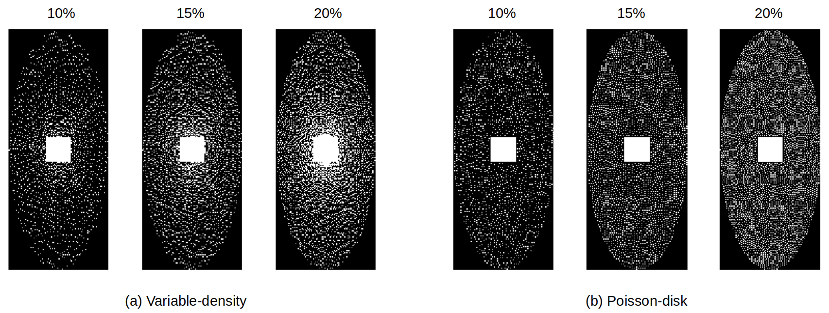
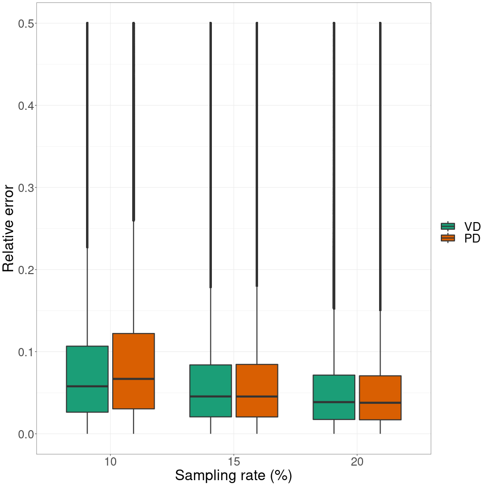
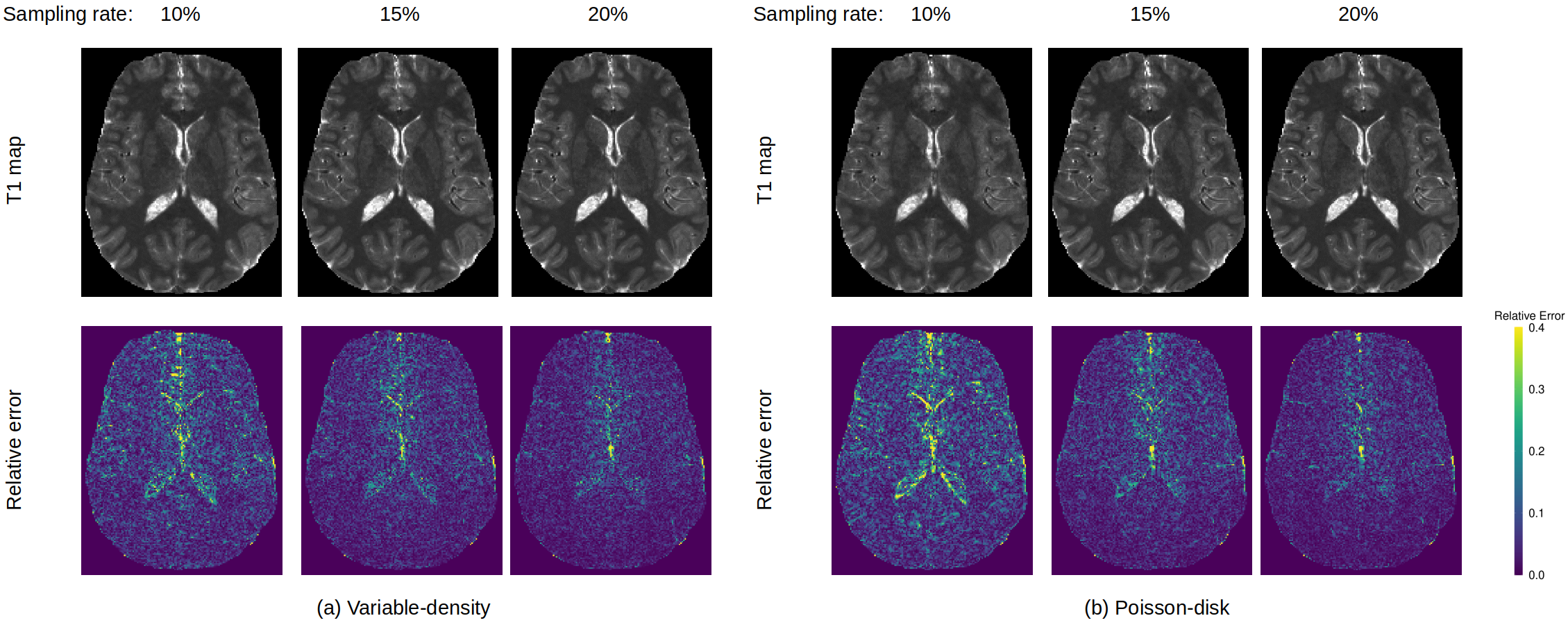
We use the proposed approach to reconstruct a $$$256\times 232\times 96$$$ in vivo brain image. The data was acquired on a 3T MRI scanner (Siemens Prisma) with a 32-channel head coil, and the k-space was fully sampled to provide the "gold standard" reference for evaluation. Measurements were acquired at three flip angles ($$$10^\circ$$$, $$$15^\circ$$$, $$$20^\circ$$$) and four echo times, where the first echo time=7ms and echo spacing=8ms, slice thickness=1.5mm, resolution=1mm, pixel bandwidth=260Hz, TR=36ms, and FoV=256mm$$$\times$$$232mm. We then performed undersampling using variable-density sampling pattern [6] and Poisson-disk sampling pattern [7], where the sampling rates varied between $$$10\%$$$ and $$$20\%$$$. The two types of sampling patterns are shown in Fig. 2, where the central $$$24\times 24$$$ k-space was always fully sampled to estimate the coil sensitivity maps. The pixel-wise relative errors in the brain region are computed and the results are shown in Fig. 3. Taking one 2D slice as an example, Fig. 4 shows the recovered T1 maps and the corresponding relative errors.

Discussion and Conclusion

We compared the performances of two undersampling patterns: variable-density (VD) and Poisson-disk (PD). We can see from Fig. 3 and 4 that VD performs better than PD when the sampling rate is very low (~$$$10\%$$$). As shown in Fig. 2, the sampling locations in VD are denser when they are closer to the center, whereas the sampling locations in PD are uniformly distributed. In general, we included more low-frequency measurements when VD was used, which proves quite beneficial when the sampling rate is low. When the sampling rate is relatively high, the two patterns perform almost equally well. In summary, we successfully applied AMP method for quantitative T1 mapping with automatic parameter estimation and inclusion of physics constrained signal model of multi-echo data, which makes it suitable for clinical T1 mapping using a prospective sampling scheme.

Acknowledgements

This work is supported by National Institutes of Health under Grants R21AG064405 and P30AG066511.