Introduction

The goal of this study is to improve the accuracy and precision of T₁ and T₂ estimations from MR Fingerprinting (MRF) by reducing thermal noise at 0.55 T. A recently introduced 0.55T system has shown potential for efficient imaging due to shorter T₁ and longer T₂/T₂* values with a reduced cost compared to higher field scanners, such as 1.5T or 3T¹. While MRF² has been shown to be an efficient and accurate method for quantifying relaxation times, the low signal-to-noise ratio (SNR) at 0.55T may reduce the accuracy and precision of T₁ and T₂, and restrict the achievable spatial resolution, reducing the potential clinical utility of this approach. Here we propose a denoising algorithm³ that matches the acquired signal to a general noise model⁴, and then removes the noise components before dictionary matching to improve the precision of MRF estimations at 0.55T.

Methods

The denoising algorithm uses a local low-rank process to decompose 3x3 voxel patches of MRF time-series data into their principal components using singular value decomposition (SVD). The generated singular values are matched to the Marcheko-Pastur (MP) distribution, a general noise model describing the singular value spectrum of random matrices. Once the noise components are identified, they are removed, and the data matrix is reconstituted without them.
Data were collected using a 2D FISP MRF sequence⁵ with variable flip angles ranging from 5° to 75°, a 1x1 mm in plane spatial resolution, a fixed TR of 18 ms, and a TE of 5.6 ms on a 0.55T scanner (MAGNETOM Siemens Free.Max Siemens Healthcare, Erlangen, Germany). 2500 time points were acquired with an acquisition time of 45 seconds for a 2D slice. Noise pre-whitening^6,7 was applied to the MRF data to remove spurious correlations between phase array coils. T₁ and T₂ maps were generated from the MRF data both before and after thermal noise removal via pattern matching using a dictionary with 10-5000 ms T₁ entries and 2-1200 ms T₂ entries with entry step size between 2-500 ms.
The T₂ layer of an ISMRM/NIST MR system phantom was scanned to assess noise removal properties. A slice thickness of 1.5 mm was used. Relaxation times from MRF were compared with reference values measured by gold standard spin-echo methods. T₂ measurements with reference values greater than 500 ms were excluded since they do not correspond to physiological values.
In vivo brain and liver data were acquired in health subjects in an IRB approved study. Brain image data was acquired with both a 5 mm and 1.5 mm slice thickness; the thinner slice was collected to assess denoising performance at extremely low SNR. Liver images were acquired with an 8 mm slice thickness.
Noise was quantified through both SNR and standard deviation, where SNR is defined as the mean divided by the standard deviation for either a single voxel across multiple scans or for a uniform group of voxels. The noise reduction was determined by comparing the SNR and standard deviation of parameter maps.
σ-normalized residuals are calculated by the difference between a parameter map and a reference sample mean from repeated measurements divided by the standard deviation of the repeated measurements. Residual maps can be thought of as error from an approximate true image. Accurate parameter maps should have a small difference with the reference and lack anatomical detail.

Results

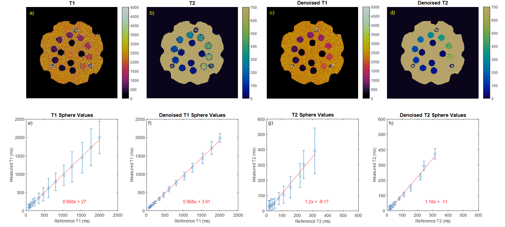
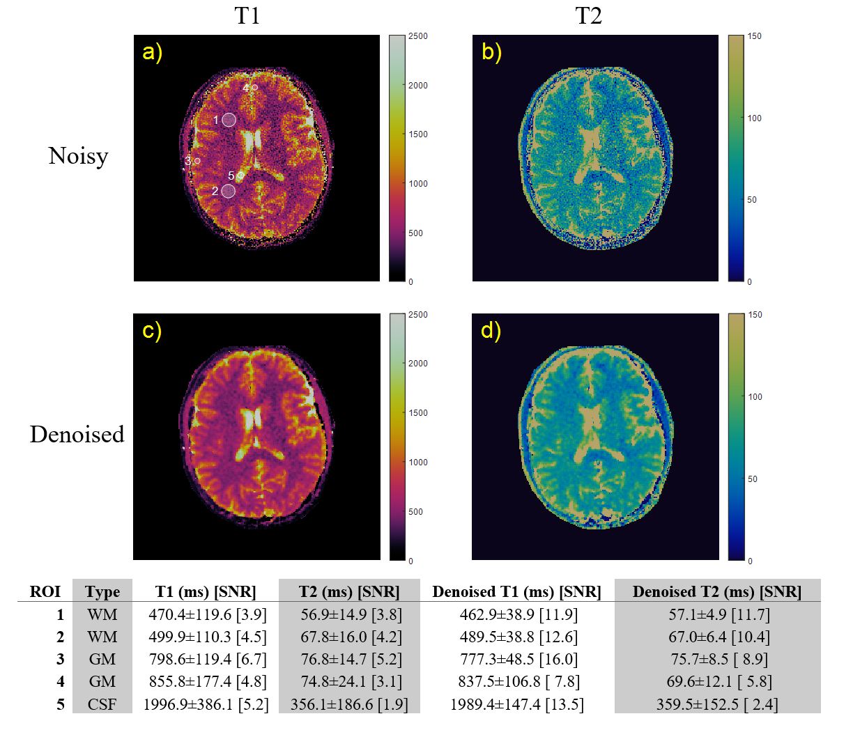
Figure 1 shows images and measured relaxation times for each sphere from the phantom data. The standard deviation, shown in the error bars, is reduced with denoising for all spheres.
Figure 2 shows denoising performance on a 1x1x5 mm resolution scan of a brain. ROIs are drawn for white matter, gray matter, and cerebrospinal fluid. Relaxation time measurements have a good agreement with results reported in literature⁸. Standard deviations are reduced by as much as a factor of 1/3rd which translates to an SNR improvement by approximately a factor of 2-3 after applying denoising. Mean measurements in each ROI typically experienced a 2% change, with only one ROI experiencing a 7% change.
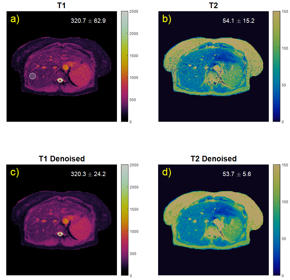
Figure 3 shows denoising performance on liver data. Relaxation time measurements within an ROI show that standard deviation is more than halved with denoising. The mean relaxation times experience less than 1 ms change with denoising.
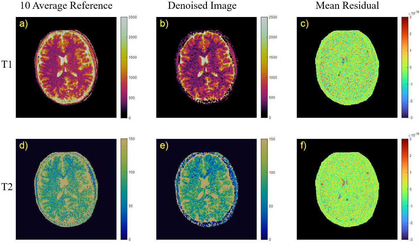
Figure 4 shows the 10-mean σ-normalized residual of denoised brain images at 1.5 mm slice thickness calculated from a 10-average reference image. The residuals contain small amounts of anatomical detail: only cerebrospinal fluid and the skull.

Discussions and Conclusions

The denoising method was shown to be effective at denoising MRF data collected at 0.55T, resulting in improved SNR and measurement precision. Denoising does not result in an improvement in measurement accuracy as the actual relaxation measurements experienced only small changes. Residuals show that denoising does not introduce much bias into the image since the residuals largely lack anatomical detail. The cerebrospinal fluid that can be seen is likely due to physiological fluctuation in the relaxation times. In the skull region, the residual shows smaller mean error, which indicates that denoising produces more precise measurements in the skull. This denoising method could be useful for improving low-field MRF and enhance the diagnostic utility of low-field MR systems.

Acknowledgements

This work was supported by Siemens Healthcare and NIH grants R37CA263583 and R01CA208236.

References

1. Runge VM, Heverhagen JT. The Clinical Utility of Magnetic Resonance Imaging According to Field Strength, Specifically Addressing the Breadth of Current State-of-the-Art Systems, Which Include 0.55 T, 1.5 T, 3 T, and 7 T. Investigative Radiology. Published online November 4, 2021. doi:10.1097/RLI.0000000000000824

2. Ma D, Gulani V, Seiberlich N, et al. Magnetic resonance fingerprinting. Nature. 2013;495(7440):187-192. doi:10.1038/nature11971

3. Veraart J, Novikov DS, Christiaens D, Ades-aron B, Sijbers J, Fieremans E. Denoising of diffusion MRI using random matrix theory. NeuroImage. 2016;142:394-406. doi:10.1016/j.neuroimage.2016.08.016

4. Marchenko V, Pastur L. Distribution of eigenvalues for some sets of random matrices. Mat Sb. 1967;72(114):507-536.

5. Jiang Y, Ma D, Seiberlich N, Gulani V, Griswold MA. MR fingerprinting using fast imaging with steady state precession (FISP) with spiral readout. Magn Reson Med. 2015;74(6):1621-1631. doi:10.1002/mrm.25559

6. Hansen MS, Kellman P. Image reconstruction: an overview for clinicians. J Magn Reson Imaging. 2015;41(3):573-585. doi:10.1002/jmri.24687

7. Kellman P, McVeigh ER. Image reconstruction in SNR units: A general method for SNR measurement†. Magnetic Resonance in Medicine. 2005;54(6):1439-1447. doi:10.1002/mrm.20713

8. Campbell-Washburn AE, Jiang Y, Körzdörfer G, Nittka M, Griswold MA. Feasibility of MR fingerprinting using a high-performance 0.55 T MRI system. Magn Reson Imaging. 2021;81:88-93. doi:10.1016/j.mri.2021.06.002