PURPOSE

Correlations between BOLD signals from a pair of gray matter (GM) cortical areas are used to infer functional connectivity but they are unable to describe how signals propagate in white matter (WM). Recently, evidence has accumulated that BOLD signals in WM are modulated by neural activities ^{1, 2}. We propose a novel analysis framework for full characterizations of information communication within the brain using fMRI signals measured from the entire cerebrum, which provides measurements of the contributions of distributed structural pathways to communications between cortical network nodes in GM, thus essentially adding a third dimension to conventional graph descriptions of brain circuits.

METHODS

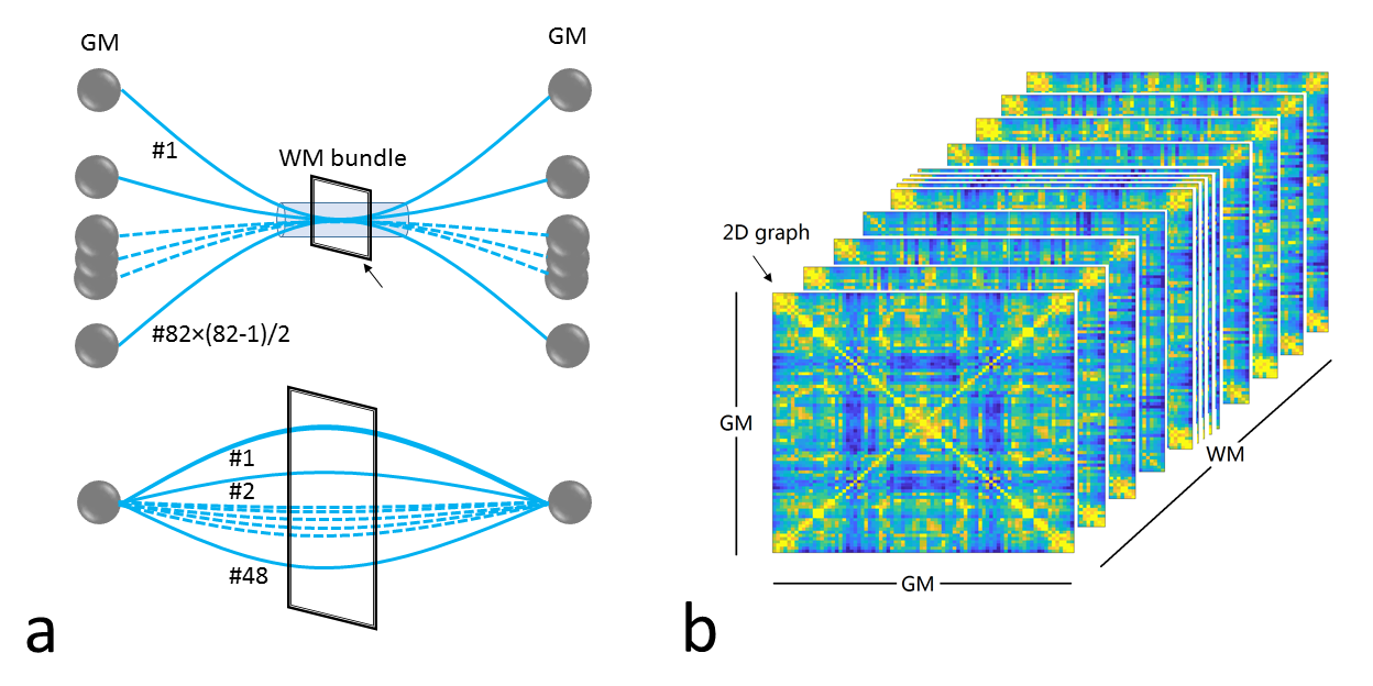
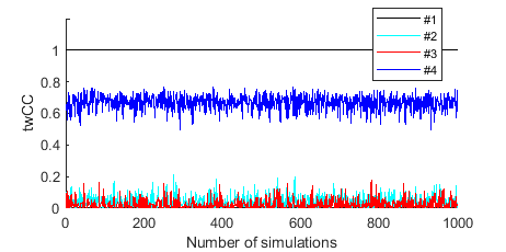
We devised a multigraph model that allows a pair of nodes to be connected by more than one edge. We parcellated GM into 82 Brodmann areas and defined 48 WM bundles in MNI space, respectively, according to the WFU PickAtlas ³ and JHU Eve atlas ⁴. We used each of the 82 Brodmann areas as a node in a multigraph model, so there are potentially 82×(82-1)/2 pairs of connected GM nodes. Each pair of nodes potentially has 48 functional routes for signal communication (i.e. edges, as shown by the blue line in the lower panel in Fig. 1a), as each of these edges goes through one WM bundle. Each WM bundle potentially contains 82×(82-1)/2 edges (as shown by the blue line in the upper panel in Fig. 1a), leading to a maximum number of 82×(82-1)/2×48 (= 94,464) combinations of signal communication units for this multigraph. This multigraph represents a complete communication model, which allows functional signals to transmit between any pair of GM regions through any WM bundles. We then defined a triple-wise correlation of fMRI signals from each pair of GM regions and one WM bundle to quantify the edge connectivity, which produces a three-dimensional GM-WM-GM correlation graph (Fig. 1b). The triple-wise correlation is achieved by first computing a matrix of covariance among the functional time series of a GM-WM-GM triplet, and then deriving eigenvalues of the covariance matrix by principal component analysis. Finally, a linear index is calculated as the difference between the two largest eigenvalues divided by the sum of all three eigenvalues. Simulations of the triple-wise correlation coefficients (twCC) reported in Fig. 2 indicate that twCC reflects the common component among a pair of GM areas and a WM bundle. In this 3D correlation graph, all twCC values in each 82×82 GM-GM 2D slice represent functional connections between all pairs of GMs (edges) through a WM bundle. Based on this 2D graph, the edge connectivity can be defined, as shown in the upper panel of Fig. 1a. To make each 2D graph more specific to its role as a part of the whole communication network, we divide the twCC values in each 2D graph by the average of the twCC values across WM bundles to remove non-specific common components. The normalized twCC in each 2D graph show variations which form a pattern. To analyze this pattern, we correlated the normalized twCC patterns with conventional GM-GM correlation maps, and call this the pattern correlation coefficient (pattern CC). We applied this approach to data from Southwest University Adult Lifespan Dataset (SALD), which were separated into 6 age groups that evenly divided the years between 20 and 80, forming group age20 through age70. The fMRI data were processed using Statistical Parametric Mapping (SPM12). Brain networks were created with binarized normalized 2D graphs with a sparsity of 0.05. The brain networks were visualized with the BrainNet Viewer ⁵.

RESULTS

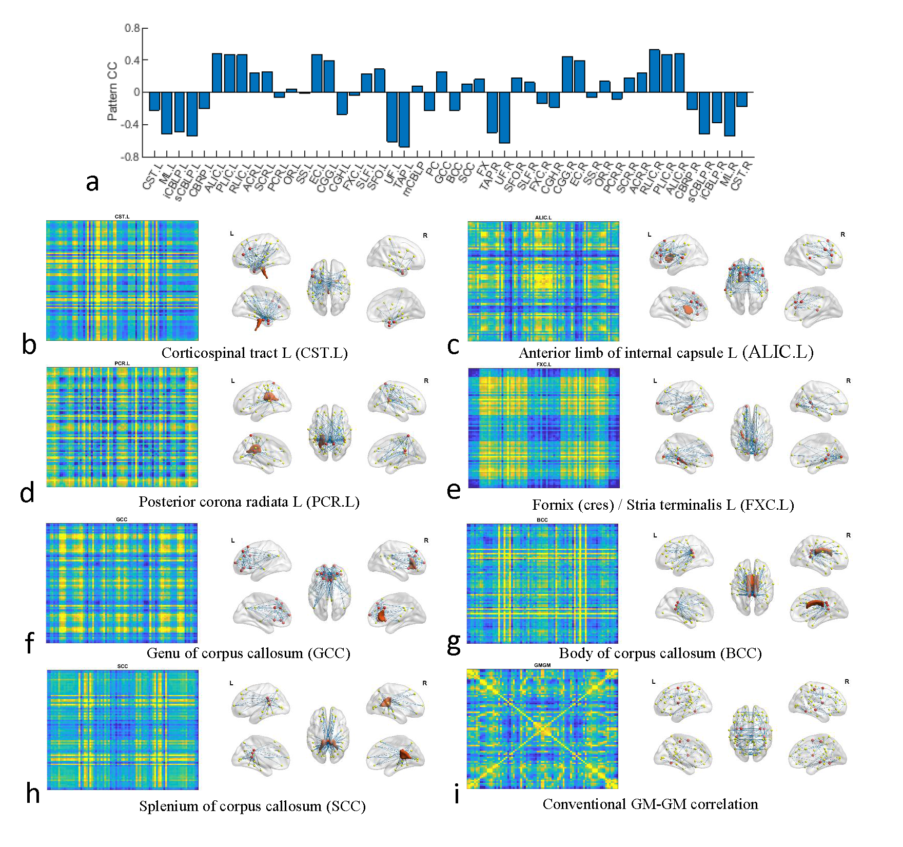
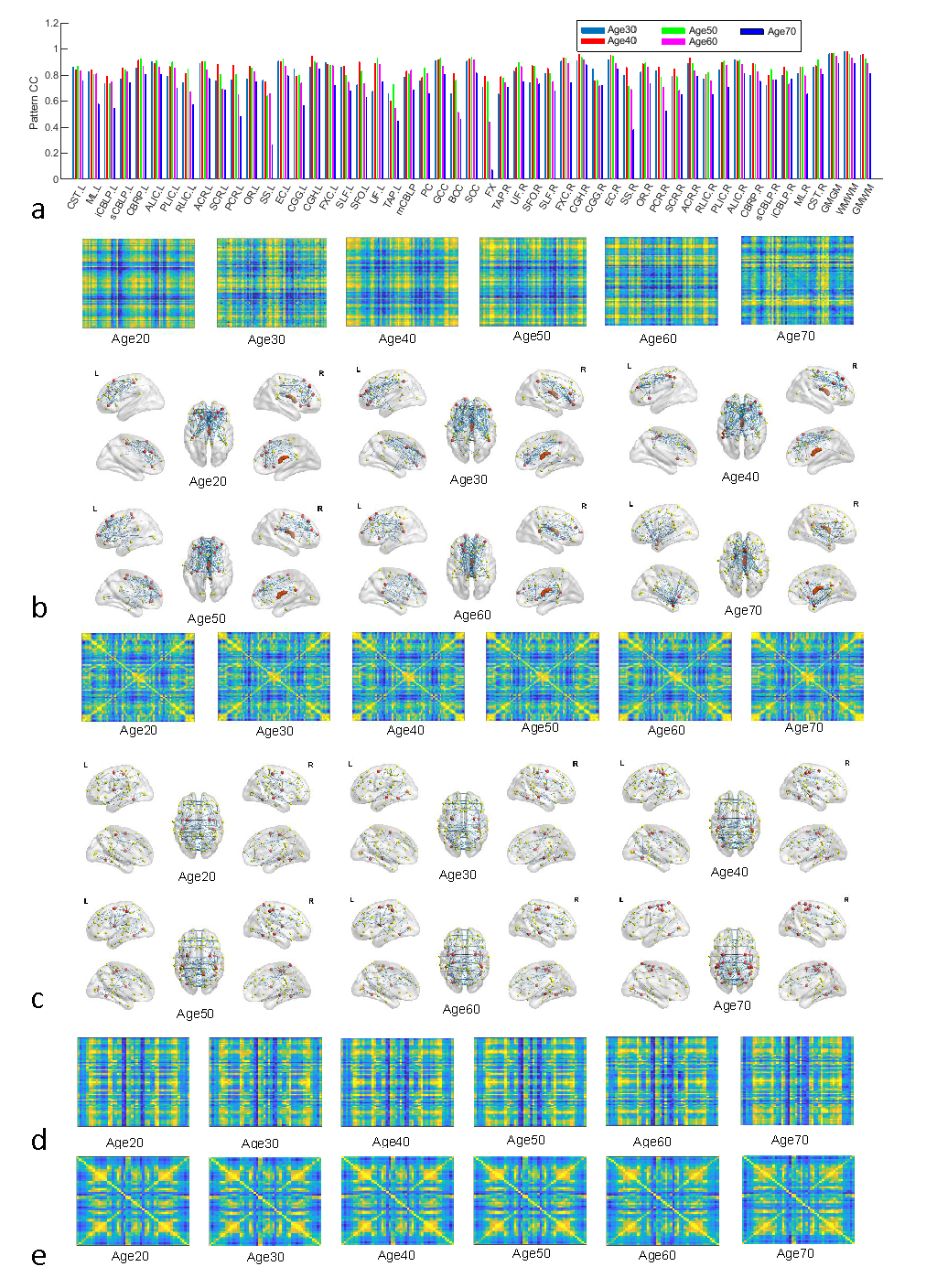
Fig. 3a shows the pattern CC between the normalized 2D graph and conventional GM-GM correlation map, which demonstrates that the normalized 2D graphs have different patterns from the conventional GM-GM correlations. Figs 3b-3i show the normalized 2D graphs or maps (left) and their corresponding brain networks (right) from several representative WM bundles and conventional GM-GM correlations for group age20. Note that the functional connections by our analysis show regional characteristics which are near a corresponding WM bundle. In contrast, the conventional GM-GM correlation shows functional connections of the whole brain. Fig. 4a shows the pattern CC of the normalized 2D graph and the conventional correlation maps of GM-GM, WM-WM, and GM-WM between several age groups, which suggests that although the conventional correlations are very high, the normalized 2D graphs for some WM bundles are relatively lower. Fig. 4b-4e show the normalized 2D graphs and/or the brain networks for WM bundle FX. Note that the structure of the functional connections through some specific WM bundles are more sensitive to age than the conventional correlations.

DISCUSSION AND CONCLUSION

Given that WM exhibits BOLD signal fluctuations similar to GM at rest, the proposed multigraph model on the basis of triple-wise correlations naturally extends current concepts for analysis of brain functional networks. Our experimental results show that it allows characterizations of functional connections between GMs through specific WM bundles.

Acknowledgements

No acknowledgement found.