3296
Normalization of conductivity maps to support identification of pathologic areas1Philips Research, Hamburg, Germany, 2Hokkaido University, Sapporo, Japan
Synopsis
Electrical tissue conductivity is an emerging quantitative diagnostic parameter, particularly for oncology. Conductivity typically increases with tumor malignancy, however, high conductivity per se is no indication for abnormal tissue, since many tissue types are highly conductive without being abnormal. An empirical rule correlates tissue conductivity with tissue water content. One possibility to analyze abnormality of tissue is thus to compare conductivity as measured with conductivity as expected from water content. The obtained difference yielding “normalized” conductivity might serve as a more direct measure of tissue abnormality. This study presents this concept using pathologic and healthy in vivo example cases.
Introduction
Electrical tissue conductivity has the potential to become a quantitative diagnostic parameter, particularly for the characterization of brain1,2 and breast tumors3,4. These studies typically show an increase of tissue conductivity with tumor malignancy. However, a high conductivity per se is no indication for abnormal tissue, i.e., many tissue types are highly conductive without being abnormal. An empirical rule correlates tissue conductivity with tissue water content W5,6. One possibility to analyze abnormality of tissue is thus to compare tissue conductivity as measured (σmeas) with tissue conductivity as expected from tissue water content (σexp). The obtained difference yielding a “normalized” conductivity σnorm = σmeas - σexp might serve as a more direct measure of tissue abnormality. In this study, the concept of normalized conductivity is presented and illustrated by in vivo cases.Theory and Methods
Electrical tissue conductivity σmeas can be estimated from the transceive phase φ of a SSFP image via σmeas(φ) = Δφ / (2μ0ω) with Δ the Laplacian operator, μ0 the magnetic vacuum permeability, and ω the Larmor frequency (“Electrical Properties Tomography”, EPT)7. The tissue water content W can be estimated from the magnitude M of a SSFP image due its joined dependence on T18. Combining these two features results in a relation σexp(M). A typical example σexp(M) for a healthy brain region is shown in Fig. 1, revealingσexp(M)=a/(1+b/(M-c)) (1)
in line with the previously reported relation M(W)5,6. Once σexp(M) is fitted, the normalized conductivity is calculated voxel-by-voxel via σnorm = σmeas - σexp as mentioned above. The three constants in Eq. (1) (a adjusting global scaling, b adjusting curvature, c adjusting shift in M direction) depend on acquisition parameters and have to be fitted for each measurement individually. Ideally, this fit is performed on the healthy part of the brain only. In practice, however, it is sufficient to perform the fit on the whole brain including both, abnormal and healthy tissue, since much less voxels with abnormal than healthy tissue are typically found, which are thus not able to alter the fit significantly.
To validate the approach, four subjects of a study published earlier were revisited1, where SSFP measurements (TR/TE = 3.5 ms/1.7 ms, α = 25°, acquired voxel size = 1.3 × 1.2 × 1 mm3, acquisition time = 3:40 min) were performed on a commercial 3T MR system (Achieva TX, Philips Medical Systems, Best, the Netherlands) with a standard 32-channel RF head coil. For subject 1 and subject 2, the approach of normalized conductivity was applied to normal-appearing brain tissue. For subject 3, the approach was applied to cystic metastasis, and for subject 4, the approach was applied to radiation necrosis and edema.
Results
Figure 2 compares σmeas , σexp , and σnorm for the two examples of normal-appearing brain regions, showing σnorm close to zero throughout the FOV. Figure 3 compares σmeas , σexp , and σnorm for the two pathologic examples, showing a pronounced increase of σnorm within the pathologic areas, while the contrast of the remaining brain structure is almost gone.Discussion
The relationship between tissue conductivity / SSFP signal on one hand and tissue water content on the other hand opens up the possibility to normalize measured conductivity by the conductivity expected empirically due to tissue water content. The resulting normalized conductivity might be able to depict pathologic tissue areas more clearly, and thus could be helpful to identify such areas.More dedicated sequences for tissue water content determination are available5, but would require additional scan time for the additional, dedicated sequence, and also bearing the risk of registration issues between the separate scans of determining conductivity and water content. In this study, SSFP has been used to estimate water content, which might be less accurate than using a dedicated sequence. However, it has the invaluable advantage that both, water content and conductivity, can be derived from the same image. Thus, the described normalization can be performed voxel-by-voxel in a straight-forward manner, and comes without additional scan time.
Conclusion
Normalizing measured tissue conductivity by the conductivity expected empirically from tissue water content has the potential to yield a new quantitative tissue parameter. Its diagnostic usefulness to support identification of pathologic areas shall be subject to future, systematic studies, also investigating the physiologic and biochemical background of the approach in more detail.Acknowledgements
The authors thank Christian Stehning for fruitful discussions.References
| 1. | Tha KK et al., Noninvasive electrical conductivity measurement by MRI: a test of its validity and the electrical conductivity characteristics of glioma. Eur Radiol. 2018;28(1):348-355. |
| 2. | Park JE et al., Low conductivity on electrical properties tomography demonstrates unique tumor habitats indicating progression in glioblastoma. Eur Radiol. 2021;31(9):6655-6665. |
| 3. | Kim SY et al. Correlation between conductivity and prognostic factors in invasive breast cancer using magnetic resonance electric properties tomography (MREPT). Eur Radiol. 2016; 26(7):2317-2326. |
| 4. | Mori N et al., Diagnostic value of electric properties tomography (EPT) for differentiating benign from malignant breast lesions: comparison with standard dynamic contrast-enhanced MRI. Eur Radiol. 2019;29(4):1778-1786. |
| 5. | Fatouros PP et al., In vivo brain water determination by T1 measurements: effect of total water content, hydration fraction, and field strength, Magn Reson Med 1991;17(2):402-413. |
| 6. | Michel E et al., Electrical conductivity and permittivity maps of brain tissues derived from water content based on T1‐weighted acquisition. Magn Reson Med. 2017;77(3):1094-1103. |
| 7. | Katscher U et al., Electric properties tomography: Biochemical, physical and technical background, evaluation and clinical applications. NMR Biomed. 2017;30(8):3729. |
| 8. | Vlaardingerbroek MT et al., Magnetic Resonance Imaging: theory and practice. Berlin: Springer; 1997. |
Figures
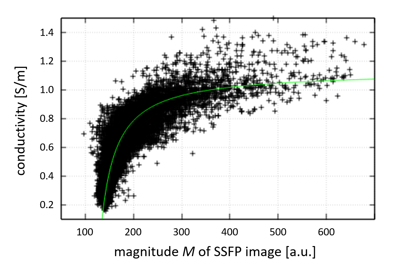
Fig. 1: Scatter plot (black data points) of a normal-appearing brain region representing measured conductivity smeas. The relationship between conductivity and SSFP magnitude image can be approximated by Eq. (1) (green line), yielding expected conductivity sexp. In this example, the constants for sexp fitted via Eq. (1) are a=1.13, b=59.7, c=265.
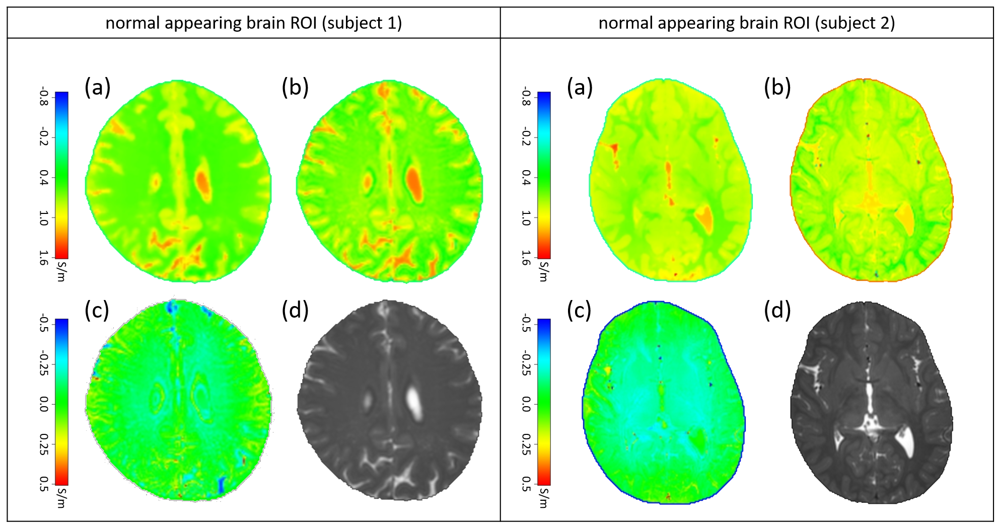
Fig. 2: Examples of normal-appearing brain regions. For both subjects, the subplots show (a) conductivity smeas derived from SSFP phase image, (b) expected conductivity sexp derived via Eq. (1), (c) difference between (a) and (b) yielding normalized conductivity snorm, which is close to zero throughout the ROIs, (d) magnitude M of SSFP image.
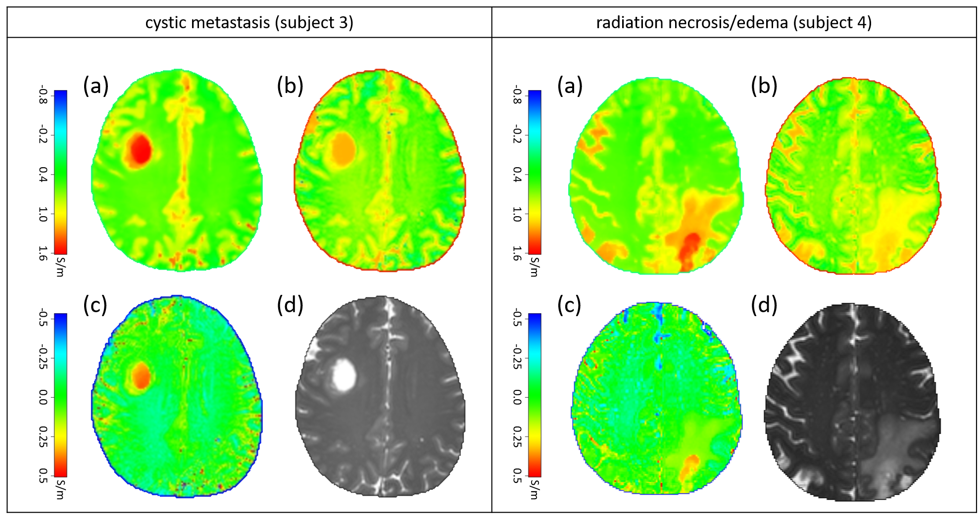
Fig. 3: Pathologic examples of normalized EPT, left: cystic metastasis, right: radiation necrosis/edema. For both patients, the subplots show (a) conductivity smeas derived from SSFP phase image, (b) expected conductivity sexp derived via Eq. (1), (c) difference between (a) and (b) yielding normalized conductivity snorm, which shows a pronounced increase within the pathological area, (d) magnitude M of SSFP image.