Introduction

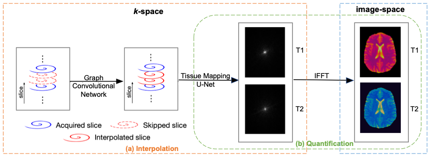
MR Fingerprinting [1] measures multiple tissue properties in a single acquisition. Compared with 2D MRF, 3D MRF provides whole-brain coverage with higher spatial resolution and SNR. However, 3D MRF, especially with an isotropic submillimeter resolution, suffers from lengthy acquisition and processing times, limiting its clinical applicability. In this work, we developed a fully deep-learning empowered pipeline consisting of (i) a graph convolutional network that replaces GRAPPA [2] for k-space interpolation and (ii) an end-to-end tissue quantification network reconstructing directly from the filled k-space data, avoiding time-consuming Non-uniform Fast Fourier Transform (NUFFT) and dictionary matching (DM). Our preliminary results show that accurate whole-brain 3D MRF acquisition with simultaneous T1 and T2 mapping with 0.8-mm isotropic resolution can be achieved in a total scan time of ~5 mins (16X acceleration: 4X along the partition and 4X along the time direction). Particularly, the reconstruction time is less than 0.5s per slice, which is ~1100 times faster than the standard NUFFT+DM reconstruction.

Methods

All MRI experiments were performed on a Siemens 3T scanner with a 32-channel receive coil. Details on the 3D MRF pulse sequence are described in [3]. The 3D MRF dataset was acquired using a stack-of-spirals trajectory. Sub-millimeter isotropic resolution was achieved via a spiral trajectory designed with a maximum gradient magnitude of 32 mT/m and a maximum slew rate of 180 mT/m/msec. Imaging parameters include: FOV, 25x25 cm; matrix size, 320x320; TR, 12.6 ms; TE, 1.3 ms; flip angles, 5-12 degrees; number of slices, 176. The acquisition time for 768 MRF time frames with 2X interleaved undersampling in k-space was ~20 min. The gold standard was obtained using GRAPPA+dictionary matching with the acquired data [3]. MRF data were acquired for 5 subjects, and 4 datasets were used for training and 1 for testing. Retrospective undersampled data were used for numerical evaluation. The total acquisition time with whole brain coverage (14 cm) was less than 5 minutes.

For training, the data underwent 4X undersampling along both the partition-encoding direction in k-space and the time dimension. Our pipeline (Fig. 1) consists of 1) a Graph Convolutional Network (GCN) for interpolating the missing k-space data, and 2) an end-to-end quantification network based on U-Net for direct tissue mapping from the interpolated spiral k-space data. Multiple time-consuming steps in the standard MRF reconstruction framework including non-uniform FFT and dictionary-based template matching are circumvented in the proposed pipeline.

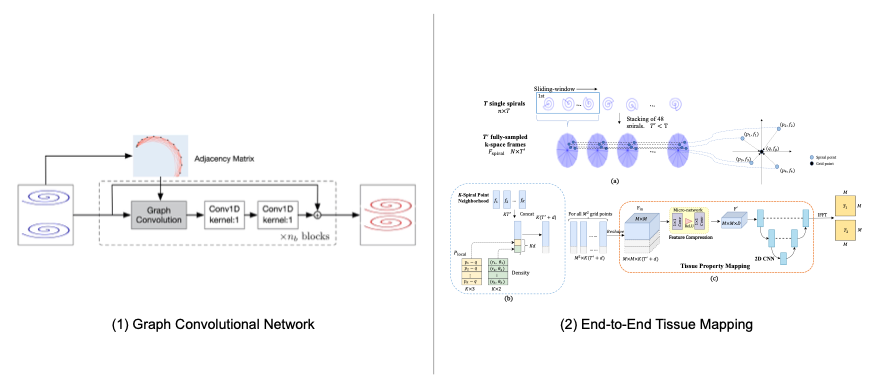
The GCN (Fig. 1(a)) [4] consists of n_b blocks where each block contains a graph convolutional layer for spatial aggregation and two 1x1 convolutional layers for feature transformation. Essentially, each block gathers local information from its 5 1-hop spiral neighbors (i.e., kernel size=5) and maps it to a new feature space for learning the correlations among the neighboring spiral points. Residual connections [5] are added to ease training. Similar to traditional parallel imaging methods [2], GCN was trained on the central k-space data containing 16 partitions.

After k-space interpolation with GCN, the data were then fed into the quantification network. Unlike the original two-stage MRF framework that first reconstructs the time frames from spiral k-space MRF data using NUFFT and then uses DM for tissue mapping, our quantification network learns end-to-end a direct mapping from the interpolated spiral k-space data to the tissue maps (Fig 1. (b)). Specifically, every T (T=32, determined by the spiral trajectory) temporally consecutive spirals were first stacked using a sliding-window for full k-space coverage. The features for each target grid point were then agglomerated from its K nearest neighbors from a stack of spirals via concatenation. Density compensation is modeled as a function of data locations on the spiral sampling trajectory, parameterized by polar coordinates of the sampled data. A U-Net [6] is employed to map the algomerated features to tissue maps so that gridding and tissue mapping are simultaneously performed from k-space. Details of the two network architectures are further described in Fig 2.

Results

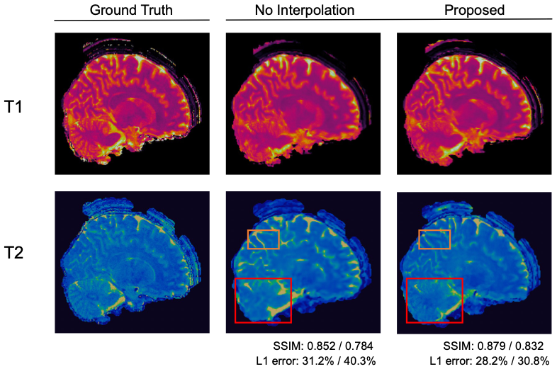
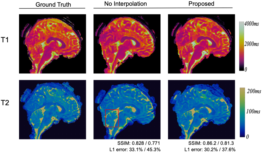
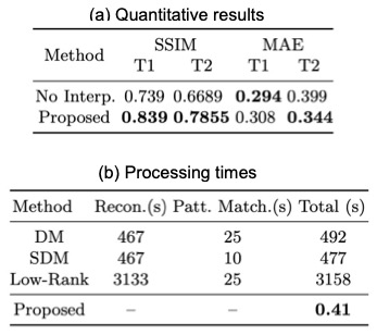
Fig. 3 and Fig. 4 show representative T1 and T2 maps of two slices obtained from the 3D MRF data with 0.8 mm isotropic resolution and 16X acceleration. Compared with no interpolation along the partitions, the proposed pipeline yields improved performance, exhibiting more details, in addition to the fast overall processing speed. Table 1 shows the quantitative results over all slices and processing times of different methods.

Discussion and Conclusion

We proposed a fully learning-based pipeline for rapid and accurate acquisition and reconstruction of high-resolution 3D MRF. We expect further boost in tissue quantification accuracy when more training data are collected in the future.

Acknowledgements

This work was supported in part by United States National Institutes of Health (NIH) grant EB006733.