3287
Alternating Joint Learning Approach for Variational Networks and Sampling Pattern in Parallel MRI1Radiology, NYU Langone Health, New York, NY, United States, 2Department of Artificial Intelligence in Biomedical Engineering, FAU Erlangen-Nuremberg, Erlangen, Germany
Synopsis
We propose a new alternating learning approach to jointly learn the sampling pattern (SP) and the parameters of a variational network (VN) for acquisition and reconstruction on 3D Cartesian parallel MRI problems. This approach is composed of alternating short training with BASS algorithm to learn the SP, and ADAM algorithm to learn the parameters of the VN, both with forced monotonicity. The results illustrate that this approach provides reduced error when compared to other joint learning approaches, and surpasses VN trained with recently developed fixed SPs.
Introduction:
Undersampling the k-space has been successfully used to accelerate MRI data acquisition, particularly when combined with parallel MRI (1,2), and special reconstructions (3–6). Compressive sensing (CS) has shown that undersampling artifacts from incoherent acquisition can be recovered with sparsity-enforced reconstructions (7). Recently, deep learning image reconstructions have shown that neural networks (NN), such as the variational networks (VN) (8), can also effectively remove artifacts from undersampled images (5,8,9). However, no specifications for the sampling pattern (SP) are currently known to be more or less effective with NN. Due to this, several approaches have been proposed to jointly learn the SP and the NN (10–12), as an attempt to understand what are the sampling requirements for effective reconstruction with NN.Here, we propose a new alternating approach to learn the SP and the parameters of a VN. The approach considers SP learning as a combinatorial problem while keeping the VN learning as regular NN training. However, forced monotonicity is used to ensure that the cost function is being reduced. Our approach shows that the learned SP and VN can surpass other jointly learned approaches, such as LOUPE (10), as well as VN learning with the most recent SPs for CS approaches, such as the Poisson-disc with variable density (PD+VD) SP (13,14).
Methods:
In the VN for undersampled parallel MRI we use the following model:$$\mathbf{m}=\mathbf{FC}\mathbf{x}.$$
In the above, $$$\mathbf{x}$$$ represents the 2D+time images, of size $$$N_x\times N_y \times N_t$$$ which denotes vertical $$$N_x$$$ and horizontal $$$N_y$$$ sizes and time $$$N_t$$$. $$$\mathbf{m}$$$ is the fully-sampled multi-coil k-t-space data. $$$\mathbf{C}$$$ denotes the coil sensitivities transform, which maps $$$\mathbf{x}$$$ into multi-coil weighted images of size $$$N_x \times N_y \times N_t \times N_c$$$, with number of coils $$$N_c$$$. $$$\mathbf{F}$$$ represents the spatial FFTs, which are $$$N_t \times N_c$$$ repetitions of the 2D-FFT.
When undersampled is used, then:
$$\bar{\mathbf{m}}=\mathbf{S}_Ω\mathbf{FC}\mathbf{x},$$
where, $$$\mathbf{S}_Ω $$$ is the sampling function using SP $$$Ω$$$ (same for all coils). The SP contains $$$M$$$ the k-t-space positions that will be sampled from a total of $$$N=N_x \times N_y \times N_t$$$ possible positions. The acceleration factor (AF) is defined as $$$N/M$$$.
In a VN (8), the reconstruction is computed by a neural network with $$$J$$$ layers that are inspired in gradient descent algorithms:
$$\mathbf{x}_{j+1} = \mathbf{x}_{j} –(\alpha_j \mathbf{C}^* \mathbf{F}^* \mathbf{S}^*_Ω(\bar{\mathbf{m}}- \mathbf{S}_Ω\mathbf{FC}\mathbf{x}_j ) + \sum_{f=1}^{N_f} \mathbf{K}^b_{j,f} \mathbf{\phi}’(\mathbf{K}_{j,f} \mathbf{x}_j )),$$
where $$$1 \leq j \leq J+1$$$ represents the layer index, where $$$J=10$$$ was used in this work.
All the VN parameters, i.e. convolutional filters $$$\mathbf{K}^b_{j,f}, \mathbf{K}_{j,f}$$$ ($$$N_f=24$$$, with complex-valued spatio-temporal filters of size $$$11×11×N_t$$$) and step-sizes $$$\alpha_j$$$, are learned from data. In this study, activation functions $$$\mathbf{\phi}’$$$ are fixed rectified linear units (ReLu).
The output of the VN can be written as:
$$\hat{\mathbf{x}}=R_{\theta}(\bar{\mathbf{m}}, Ω),$$
where $$$R_{\theta}$$$ represents the VN with parameters $$$\theta = \left\{ \left\{ \mathbf{K}^b_{j,f}, \mathbf{K}_{j,f},\right\}_{f=1}^{N_f} , \alpha_j \right\}_{j=1}^J$$$.
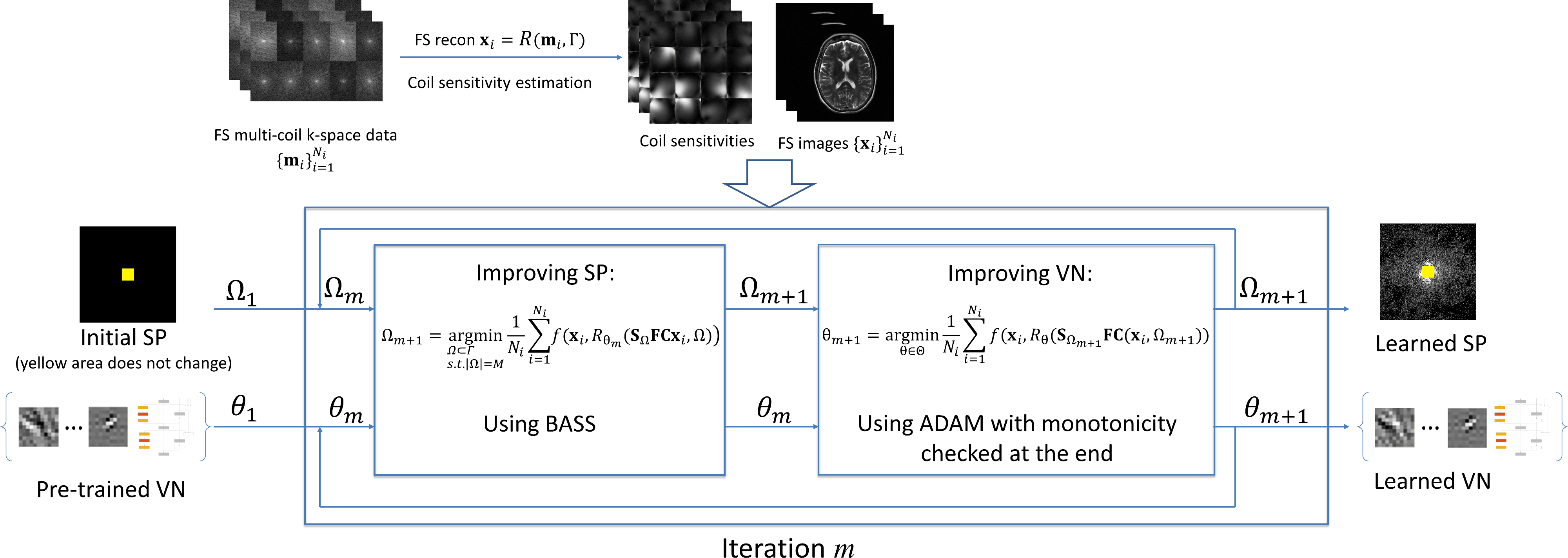
Our proposed approach, illustrated in Fig. 1 formulates the joint learning problem as an alternating minimization problem:
$$ Ω_{m+1} =\arg\min_{ \begin{array}{c}Ω \subset \Gamma\\ s.t. |Ω|=M\end{array}} \frac{1}{N_i} \sum_{i=1}^{N_i} f(\mathbf{x}_i , R_{\theta_m}( \mathbf{S}_Ω\mathbf{FC}\mathbf{x}_i, Ω).$$
$$ \theta_{m+1} = \arg\min_{ \theta \in \Theta} \frac{1}{N_i} \sum_{i=1}^{N_i} f(\mathbf{x}_i , R_{\theta}( \mathbf{S}_{Ω_{m+1}} \mathbf{FC}\mathbf{x}_i, Ω_{m+1})).$$
In the equations above, $$$ N_i$$$ is the number of images used for training. To learn the SP, some iterations of BASS (15) are used ($$$K_{init}=512$$$, $$$\alpha=0.5$$$, and stops when $$$K=1$$$), while to learn the VN parameters, some iterations of ADAM (16) are used ($$$8$$$ epochs with initial learning-rate of $$$2\times10^{-4}$$$, with a learning-rate drop factor of $$$0.25$$$, applied every $$$2$$$ epochs, and batch size of $$$8$$$ images). Monotonicity is forced in both algorithms.
We compared the proposed approach against LOUPE (10), modified for parallel MRI (17), and a VN using a fixed PD+VD SP (13). All learning approaches started with pre-trained VN ($$$80$$$ epochs, ADAM algorithm, with an initial learning-rate of $$$2\times10^{-4}$$$, learning-rate drop factor of $$$0.5$$$ applied every $$$5$$$ epochs, and batch size of $$$8$$$ images), trained with diverse SPs and diverse AFs. Because LOUPE learns a sampling density (SD) instead of an SP, we retrained the VN with one randomly generated SP from the learned LOUPE SD.
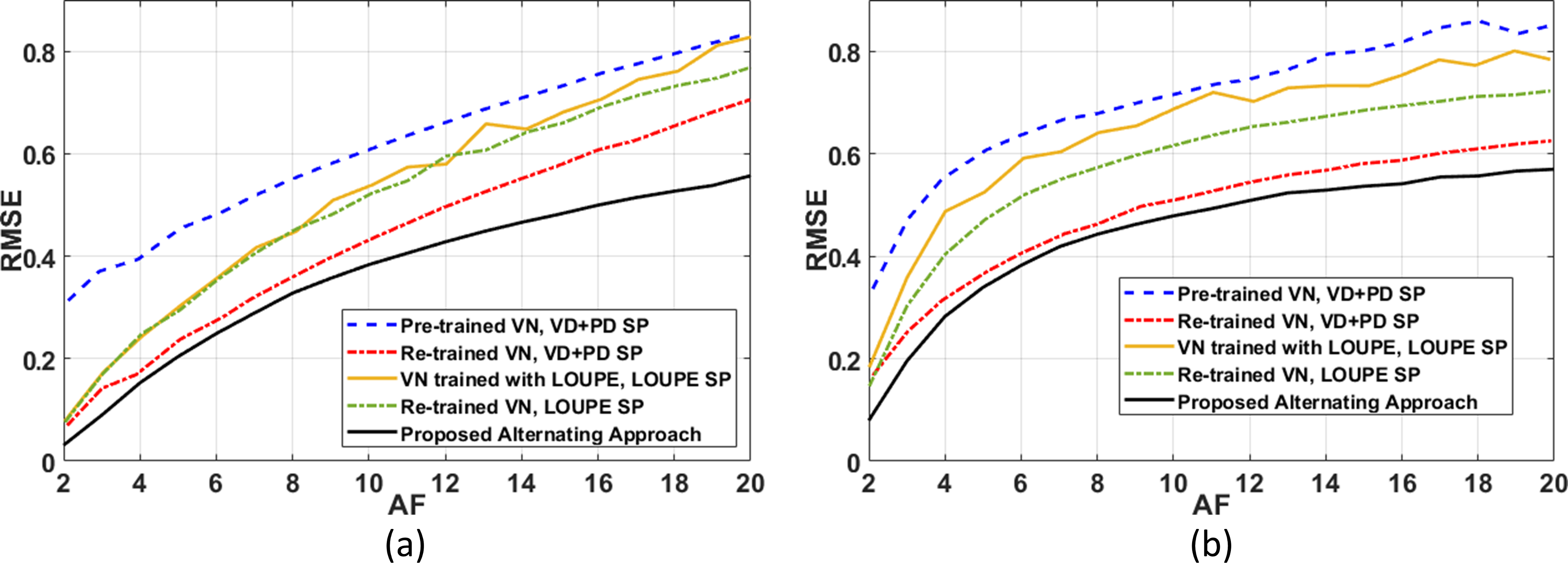
We assessed the root mean squared error (RMSE) on two datasets: brain and knee. The brain dataset contains $$$260$$$ images of size $$$N=320 \times 320 \times 1$$$ for training and $$$60$$$ for testing. The knee dataset contains the same number of images of size $$$N=128 \times 64 \times 10$$$ that is used for T1ρ mapping (18,19).
Results and Discussion:
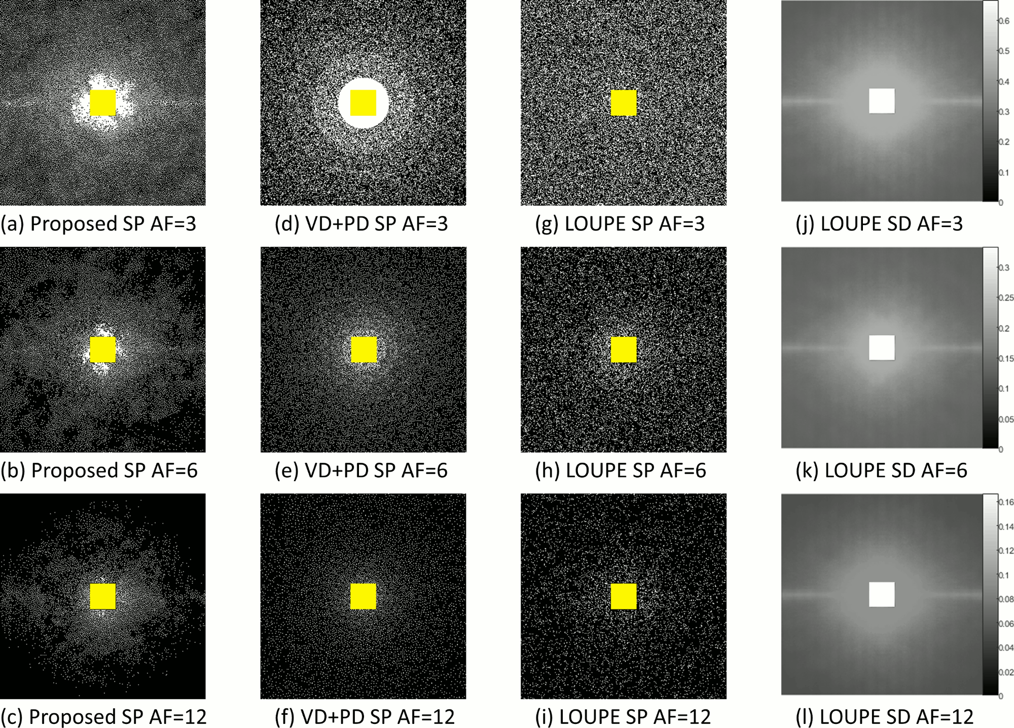
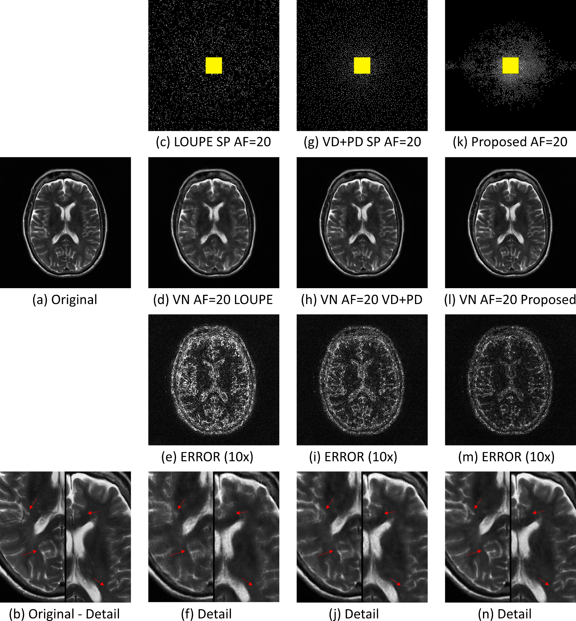
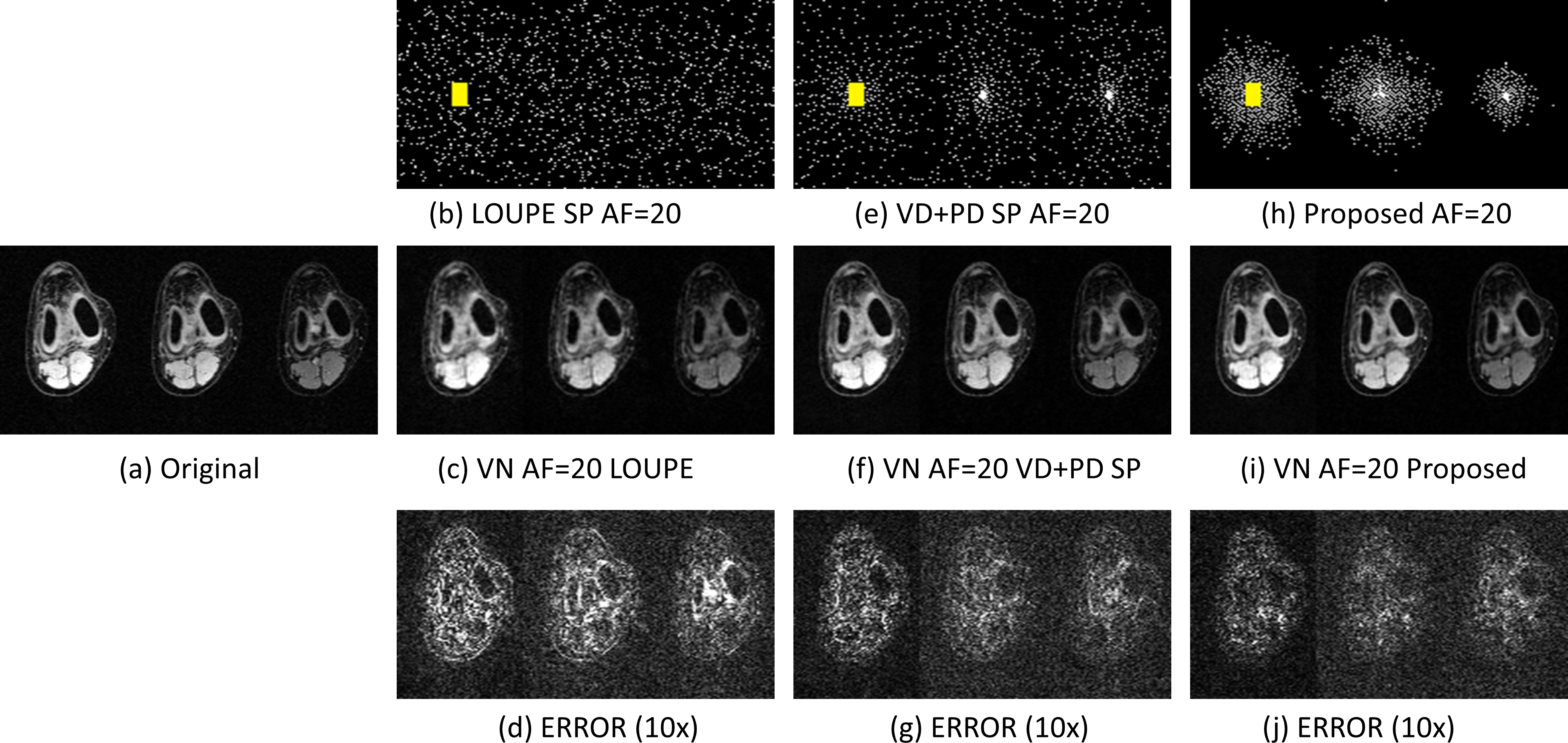
In Fig. 2 the resulting RMSE for both datasets at different AF is shown. Note that the proposed approach achieved better RMSE than the other approaches (between $$$14.9%\~51.2%$$$). A comparison between the learned SPs is shown in Fig. 3. Note that the proposed approach learned the low and mid frequencies are more important to be sampled.In Fig. 4, some visual examples with the brain dataset are shown. Note that the proposed approach seems less noisy and recovered some structures better. In Fig. 5, some results for the knee dataset are shown. In this example, the ability to learn temporal sampling is also shown.
Conclusion
Our alternating learning approach showed improvements in accelerated MRI when compared to other joint learning approaches or VN trained with fixed SPs.Acknowledgements
This study was supported by NIH grants, R21-AR075259-01A1, R01-AR068966, R01-AR076328-01A1, R01-AR076985-01A1, and R01-AR078308-01A1 and was performed under the rubric of the Center of Advanced Imaging Innovation and Research (CAI2R), an NIBIB Biomedical Technology Resource Center (NIH P41-EB017183).References
1. Ying L, Liang Z-P. Parallel MRI Using Phased Array Coils. IEEE Signal Process. Mag. 2010;27:90–98 doi: 10.1109/MSP.2010.936731.
2. Blaimer M, Breuer F, Mueller M, Heidemann RM, Griswold MA, Jakob PM. SMASH, SENSE, PILS, GRAPPA. Top. Magn. Reson. Imaging 2004;15:223–236 doi: 10.1097/01.rmr.0000136558.09801.dd.
3. Tamir JI, Ong F, Anand S, Karasan E, Wang K, Lustig M. Computational MRI With Physics-Based Constraints: Application to Multicontrast and Quantitative Imaging. IEEE Signal Process. Mag. 2020;37:94–104 doi: 10.1109/MSP.2019.2940062.
4. Feng L, Benkert T, Block KT, Sodickson DK, Otazo R, Chandarana H. Compressed sensing for body MRI. J. Magn. Reson. Imaging 2017;45:966–987 doi: 10.1002/jmri.25547.
5. Knoll F, Hammernik K, Zhang C, et al. Deep-learning methods for parallel magnetic resonance imaging reconstruction: A survey of the current approaches, trends, and issues. IEEE Signal Process. Mag. 2020;37:128–140 doi: 10.1109/MSP.2019.2950640.
6. Jacob M, Ye JC, Ying L, Doneva M. Computational MRI: Compressive Sensing and Beyond [From the Guest Editors]. IEEE Signal Process. Mag. 2020;37:21–23 doi: 10.1109/MSP.2019.2953993.
7. Lustig M, Donoho DL, Santos JM, Pauly JM. Compressed sensing MRI. IEEE Signal Process. Mag. 2008;25:72–82 doi: 10.1109/MSP.2007.914728.
8. Hammernik K, Klatzer T, Kobler E, et al. Learning a variational network for reconstruction of accelerated MRI data. Magn. Reson. Med. 2018;79:3055–3071 doi: 10.1002/mrm.26977.
9. Liang D, Cheng J, Ke Z, Ying L. Deep magnetic resonance image reconstruction: Inverse problems meet neural networks. IEEE Signal Process. Mag. 2020;37:141–151 doi: 10.1109/MSP.2019.2950557.
10. Bahadir CD, Wang AQ, Dalca A V., Sabuncu MR. Deep-Learning-Based Optimization of the Under-Sampling Pattern in MRI. IEEE Trans. Comput. Imaging 2020;6:1139–1152 doi: 10.1109/TCI.2020.3006727.
11. Aggarwal HK, Jacob M. J-MoDL: Joint Model-Based Deep Learning for Optimized Sampling and Reconstruction. IEEE J. Sel. Top. Signal Process. 2020;14:1151–1162 doi: 10.1109/JSTSP.2020.3004094.
12. Weiss T, Vedula S, Senouf O, Michailovich O, Zibulevsky M, Bronstein A. Joint Learning of Cartesian under Sampling and Reconstruction for Accelerated MRI. In: IEEE International Conference on Acoustics, Speech and Signal Processing. Vol. 2020-May. IEEE; 2020. pp. 8653–8657. doi: 10.1109/ICASSP40776.2020.9054542.
13. Levine E, Daniel B, Vasanawala S, Hargreaves B, Saranathan M. 3D Cartesian MRI with compressed sensing and variable view sharing using complementary poisson‐disc sampling. Magn. Reson. Med. 2017;77:1774–1785 doi: 10.1002/mrm.26254.
14. Dwork N, Baron CA, Johnson EMI, O’Connor D, Pauly JM, Larson PEZ. Fast variable density Poisson-disc sample generation with directional variation for compressed sensing in MRI. Magn. Reson. Imaging 2021;77:186–193 doi: 10.1016/j.mri.2020.11.012.
15. Zibetti MVW, Herman GT, Regatte RR. Fast data-driven learning of parallel MRI sampling patterns for large scale problems. Sci. Rep. 2021;11:19312 doi: 10.1038/s41598-021-97995-w.
16. Kingma DP, Ba J. Adam: A Method for Stochastic Optimization. arXiv Prepr. 2014:1–15.
17. Zhang J, Zhang H, Wang A, et al. Extending LOUPE for K-Space Under-Sampling Pattern Optimization in Multi-coil MRI. Lect. Notes Comput. Sci. (including Subser. Lect. Notes Artif. Intell. Lect. Notes Bioinformatics) 2020;12450 LNCS:91–101 doi: 10.1007/978-3-030-61598-7_9.
18. Zibetti MVW, Sharafi A, Otazo R, Regatte RR. Accelerating 3D-T1ρ mapping of cartilage using compressed sensing with different sparse and low rank models. Magn. Reson. Med. 2018;80:1475–1491 doi: 10.1002/mrm.27138.
19. Zibetti MVW, Johnson PM, Sharafi A, Hammernik K, Knoll F, Regatte RR. Rapid mono and biexponential 3D-T1ρ mapping of knee cartilage using variational networks. Sci. Rep. 2020;10:19144 doi: 10.1038/s41598-020-76126-x.
Figures