3280
Automatic parameter selection for quantitative susceptibility mapping (QSM) with regard to Shearlet/TGV-regularization
Janis Stiegeler1,2 and Sina Straub1
1Medical Physics in Radiology, German Cancer Research Center (DKFZ), Heidelberg, Germany, 2Department of Physics and Astronomy, University of Heidelberg, Heidelberg, Germany
1Medical Physics in Radiology, German Cancer Research Center (DKFZ), Heidelberg, Germany, 2Department of Physics and Astronomy, University of Heidelberg, Heidelberg, Germany
Synopsis
In this work noise is assumed to be a random vector and the method of unbiased predictive risk estimator (UPRE) is used to select suitable data/regularization parameters to solve the local phase to susceptibility deconvolution problem of quantitative susceptibility mapping (QSM). The proposed algorithm is tested on the simulated multi-echo data provided at the 2019 QSM Reconstruction Challenge. This work is a further development of the algorithm presented at the ISMRM Meeting 2021 and its purpose is to show that the method of UPRE can be applied advantageously to a shearlet /TGV based susceptibility reconstruction.
Introduction
The choice of the optimal parameters is a major problem of optimization based approaches to solve inverse problems such as the local phase to susceptibility deconvolution for QSM. However, in real clinical scenarios these parameters have always to be selected automatically to avoid time consuming and unfended trials. In this work noise is assumed to be a random vector and the method of unbiased predictive risk estimator (UPRE) is used to select suitable parameters. The proposed algorithm is tested on the simulated multi-echo data provided at the 2019 QSM Reconstruction Challenge (RC2)1. This work is a further development of the algorithm presented at the ISMRM Meeting 20212 and its purpose is to show that the method of UPRE can be applied advantageously to a shearlet /TGV based susceptibility reconstruction.Theory
The inverse problem, typically solved to obtain the susceptibility map $$$\chi$$$ from the local phase $$$\psi$$$, can be formulated in Fourier space as : $$ \mathcal{F}(\psi) (\textbf{k}) = D(\textbf{k}) \mathcal{F}(\chi) (\textbf{k}) , \quad \textbf{k} = (k_x,k_y,k_z) \in \mathbb{R}^3. $$ Here $$$\mathcal{F}$$$ denotes the Fourier transform, and $$$D$$$ the dipole kernel: $$ D(\textbf{k}) := \frac{1}{3}- \frac{k_z^2}{|\textbf{k}|^2}. $$ To achieve a unique solution without artifacts, the shearlet transform3 of the to be determined $$$\chi$$$ and a TGV-term are used as regularizers2. The method of alternating direction of multipliers (ADMM) is applied to solve the resulting optimization problem containing two data-fit terms and the two regularization terms2,4. Therefore, auxillary variables $$$w,d,t,b^w,b^d,b^t$$$ and three new parameters $$$\mu =(\mu_1,\mu_2,\mu_3) > 0$$$ are introduced and the problem is split into multiple subproblems which are easier to solve2,5,6,7 :$$ \begin{split} \chi_{k+1} &= \text{arg}\min_ {\chi}\:\frac{\beta_1}{2} ||E\chi-\psi||_2^2 + \frac{\beta_2}{2} || \chi_{well}- Mx||_2^2 + \frac{\mu_1}{2} ||w_k - \Psi \chi – b^w_k||_2^2 + \frac{\mu_2}{2} ||d_k – (\nabla^f \chi – v) – b^d_k||_2^ +\frac{\mu_3}{2} ||t_k -\zeta^bv – b^t_k||_2^2 2, \quad (1) \\ w_{k+1} + &= \text{arg}\min_w \: ||w||_1 + \frac{\mu_1}{2} ||w - \Psi \chi_{k+1} – b^w_k||_2^2,\\ d_{k+1} + &= \text{arg}\min_d \: ||d||_1 + \frac{\mu_2}{2} ||d – (\nabla^f \chi_{k+1} – v_{k+1}) – b^d_k) – b^d_k||_2^2,\\ t_{k+1} + &=\text{arg}\min_t: ||t||_1 + \frac{\mu_3}{2} ||t – \zeta^bv_{k+1} – b^t_k ||_2^2 ,\\ b^w_{k+1} &= b^w_k + \Psi \chi_{k+1} - w_{k+1}, \\ b^d_{k+1} &= b^d_k + (\nabla^f \chi_{k+1} - v_{k+1} )- d_{k+1}, \\ b^t_{k+1} &= b^t_k + \zeta v_{k+1} - t_{k+1}, \end{split}. $$ To determine suitable parameters $$$\alpha = \beta_{1,2},\mu_{2,3}$$$ one by one (whereby the other unknown parameters are set to zero and $$$\mu_1$$$ is set as an upper limit of the shearlet coefficients of a LSQR solution $$$\chi_{LSQR}$$$), the predictive risk $$$\frac{1}{n}||p_\alpha||_2^2 = \frac{1}{n}||K\chi_{\alpha}-K \chi_{true})||_2^2$$$ with the true susceptibility map $$$\chi_{true}$$$ and the regularized solution $$$\chi_{\alpha}$$$ is estimated8 and paramters were chosen to minimize the unbiased predictive risk estimator $$$U$$$.Here $$$K = \mathcal{F}^*\tilde{D}(\textbf{k}) \mathcal{F}$$$ and $$$\tilde{D}$$$ is the pointspread function of the respective data term, e.g. $$$\tilde{D} = D$$$ for the determination of $$$\beta_1$$$.
Methods
The RC2 provided simulated local phase data related to two different susceptibility ground truths (Sim1/2) and different error metrics1. Phase data from different echoes were combined after weighting with the inverse standard deviation of the noise of the phase data and a laplacian based suppression of phase errors for each echo. Noise was assumed to be a random vector such that related quantities like $$$\psi$$$ and $$$\chi_{\alpha}$$$ and the predictive risk were also random vectors or variables. As equation (1) can be solved by diagonalization in Fourier space the regularized solution $$$\chi_{\alpha} = R_{\alpha} d$$$, where $$$R_{\alpha}$$$ is a linear regularization operator and $$$d = \psi$$$ for all but the determination of $$$\beta_2$$$ - in that case $$$d = \chi_{well}$$$2,4. With $$$A_{\alpha}=KR_{\alpha}$$$ the predictive error can be split into a deterministic and a stochastic term: $$p_{\alpha}=(A_\alpha-I)K\chi_{true} + A_{\alpha}\eta.$$ Here $$$\eta$$$ is the noise vector. Since $$$A_{\alpha}$$$ is selfadjoint and noise is approximately Gaussian distributed (for high SNR in the magnitude image), neglecting covariance terms in the case of determining $$$\beta_2$$$ and by approximating the voxelwise variance $$$\sigma^2$$$ by the mean of the VOI, the UPRE $$$U$$$ can be expressed via the regularized residuum $$$r_{\alpha}$$$8: $$U(\alpha) = \frac{1}{n}||r_{\alpha}||_2^2 + \frac{2 \text{mean}(\sigma^2)}{n}\text{trace}(A_{\alpha})-\text{mean}(\sigma^2).$$ The suitable regularization parameter is then obtained by finding the roots of the derivative of $$$U$$$ with the Matlab function fzero. To determine $$$\mu_{2,3}$$$ only the data term with the local phase $$$\psi$$$ was considered. Finally, by solving $$ \tilde{s} = \text{arg}\min_s U_1(s \beta_1 )+U_2((1-s)\beta_2)$$ the scale factor $$$\tilde{s}$$$ was determined and parameters were updated to:$$\begin{align} \tilde{\beta}_1 &= \tilde{s} \beta_1,\\ \tilde{\beta}_2 &= (1-\tilde{s}) \beta_2\\ \tilde{\mu}_{2,3} &= \tilde{s} \mu_{2,3}. \end{align}$$.
Results and Discussion
Table 1 shows the achieved image quality measures (IQM) for the susceptibility maps of the proposed algorithm (PA) and the winner algorithms of RC2 in the Robustness/RMSE category (mcTFI9 /wL1L2TV10).The PA achieves a top ranking except for the streaking error. The just mentioned susceptibility maps (related to the susceptibility model Sim2) are shown in Figure 1. The good IQM achieved by the PA and the visual appearance of the obtained QSM verify that the UPRE method is suitable for automatic parameter selection. The purpose of this work is to show that the UPRE method can be applied within a susceptibility map reconstruction algorithm, using the benefits of shearlets and TGV, to find suitable regularization parameters.Acknowledgements
This work was supported by a grant from Deutsche Forschungsgemeinschaft (Grant number: DFG STR 1480/2-1). The use of the data from the 2019 Reconstruction Challenge is kindly acknowledged. The use of code for the shearlet reweighing provided by Dr. Jackie Ma is kindly acknowledged as well as the use of the code for the shearlet transform from ShearLab3D.References
- QSM Challenge 2.0 Organization Committee, Bilgic, B, Langkammer, C, Marques, JP, Meineke, J, Milovic, C, Schweser, F. QSM reconstruction challenge 2.0: Design and report of results. Magn Reson Med. 2021; 86: 1241- 1255. https://doi.org/10.1002/mrm.28754
- J. Stiegeler and S. Straub, Shearlet-based susceptibility map reconstruction with additional TGV-regularization, ISMRM & SMRT Virtual Conference & Exhibition, 15-20 May 2021.
- G. Kutyniok, W.-Q. Lim, R. Reisenhofer, ShearLab 3D: Faithful Digital Shearlet Transforms Based on Compactly Supported Shearlets. ACM Trans. Math. Software 42 (2016), Article No.: 5. www.shearlab.org.
- Kames C. et al., Rapid two-step dipole inversion for susceptibility mapping with sparsity priors. NeuroImage Volume 167, 15 February 2018, Pages 276-283.
- Candès E. J. et al., Enhancing sparsity by reweighted $l_1$ minimization. J. Fourier Anal. Appl., vpl. 14, no. 5-6, pp. 877-905, 2008
- Ma J. and März M., A multilevel based reweighting algorithm with joint regularizers for sparse recovery. arXiv:1604.06941 [math.OC], 2017.
- Ma J. et al.,Shearlet-based compressed sensing for fast 3D cardiac MR imaging using iterative reweighting. Physics in Medicine and Biology (2018). 63. 235004. 10.1088/1361-6560/aaea04.
- Vogel C. R., Computational methods for Inverse Problems. Frontiers in applied mathematics (SIAM), ISBN 978-0-898715-50-7
- Wen Y, Nguyen T, Cho J, Spincemaille P, Wang Y. Improved sig-nal modeling in quantitative susceptibility mapping using multi- echo complex Total Field Inversion (mcTFI). In Proc. Intl. Soc. Mag. Reson. Med. 2020, p. 3200
- Lambert M, Milovic C, Tejos C. Hybrid data fidelity term ap-proach for quantitative susceptibility mapping. In Proc. Intl. Soc. Mag. Reson. Med. 2020, p. 3205.
Figures
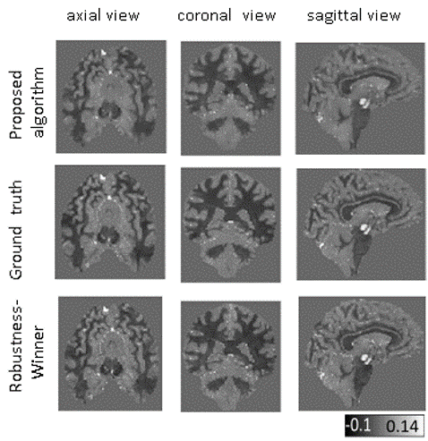
Fig 1: In the first row the susceptibility map (calcualated from the dataset related to Sim2) obtained by the proposed algorithm (PA) is shown. The second row shows the ground truth (Sim2) and in the third row the susceptibility map of the winner of RC2 in the Robustness category (mcTFI)1,9 is shown (also calculated from the dataset related to Sim2).
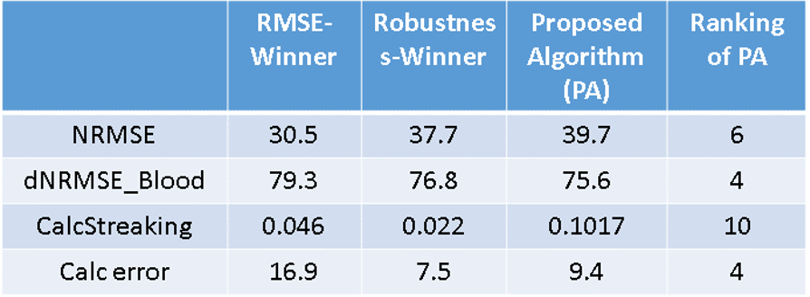
Tab 1 The values of selected IQM achieved by the QSM obtained by the proposed algorithm (PA) and by the winner algorithms of RC2 in the Robustness/RMSE category are shown in the first and second column. The third column shows the achieved ranking in RC2 compared to the top 10 scoring algorithm in the category NRMSE. NRMSE is the normalized RMSE. d_NRMSE_blood is the demeaned and detrended NRMSE for blood regions. CalcStreaking measures the error inside a neighborhood surrounding the calcification. Calc error measures the error in the quantification of the total moment of the calcification
DOI: https://doi.org/10.58530/2022/3280