3258
Observing Clearance Pathway in Alzheimer Patients Using T2 Component Analysis1Department of Radiology, Juntendo University, Tokyo, Japan, 2Canon Medical Systems Corporation, Otawara, Japan, 3Neurosurgery, Kugayama Hospital, Tokyo, Japan, 4Department of Neurosurgery, Juntendo University, Tokyo, Japan, 5Department of Neurosurgery, Juntendo Tokyo Koto Geriatric Medical Center, Tokyo, Japan, 6Department of Neurosurgery, Junterndo Tokyo Koto Geriatric Medical Center, Tokyo, Japan
Synopsis
A method to visualize possible waste clearance pathway in the brain was proposed earlier. The method is based on an assumption that there exist water containing macromolecules along the clearance pathway, and this water can be visualized using T2 component analysis. Preliminary results of this method applied for Alzheimer patients, as well as healthy volunteers, are presented. Distinct differences between the patients and healthy volunteers were observed. It is expected that this method can be a powerful tool for understanding the patho-physiology of the Alzheimer disease.
Introduction
As waste clearance system in the brain, a number of hypotheses have been proposed, e.g., the glymphatic system (1) and the intramural peri-arterial drainage (IPAD) system (2). Currently existing imaging methods include: intrathecal gadolinium injection (3), intravenous gadolinium injection (4, 5), and diffusion based analyses (6, 7). However, direct visualization in human subjects have not been achieved so far. An indirect method for this purpose was proposed by our group (8). In this method, the decaying MR signal is decomposed into different components with distinct T2 value. Assuming there exists extra-cellular water containing macro molecule waste products along the clearance pathway, this pathway, or at least its candidate can be visualized. This method does not depend on tracers, and obtains information on water and solutes in the brain. Although this method measures a steady-state data, it is possible to estimate water dynamics by comparing different steady-state data in pathological conditions and healthy physiological condition. In this work, we compared the results for Alzheimer patients and heathy volunteers.Methods
1) MR imaging Multi-echo images were acquired using a CPMG (Curr, Purcell, Meiboom, Gill) imaging sequence on a 3T clinical scanner (Canon Medical Systems). Non-selective inversion pulses were used. Also, flow compensation along SI direction and fat suppression were turned on. Imaging parameters were as follows: TR = 5000 msec, the echo interval was 40 msec, slice thickness = 4mm, number of echoes was 25, TE = 40, 80, 120, ..., 1000 msec (Fig 1).2) NNLS (non-negative least squares) The decaying signal was decomposed into 25 T2 components between 60 and 2000 msec, using NNLS in pixel by pixel basis (Fig 2). Standard Lawson and Hanson algorithm (9) was used for NNLS (8).
3) Quantification and color map After NNLS, each pixel will have 25 T2 values. In order to analyze this data in a meaningful way, a fuzzy classification, allowing overlap between components, was applied to each pixel data. Empirical probability density curves were created for each of intra-cellular water, extra-cellular water, and cerebrospinal fluid (CSF), allowing overlap between tissues. Direct result of this classification are 3 images representing intra- and extra-cellular water, and CSF. From these images, quantitative measures, like fraction and average T2 value for each component can be calculated. It is also possible to assign different color for each component and add RGB values for each pixel to generate a color map for visual inspection (Figs 3, 4).
4) Clinical protocol After IRB approval of our institution, volunteers and patients data were acquired and processed according to above mentioned method. The numbers of subjects are 4 volunteers and 10 patients, as of this abstract, and increasing at a pace of about two cases per week. Since this is a single slice method, a pre-determined slice location was applied to every patient (Fig 5).
Results and discussion
Result of NNLS is shown in fig 2. Although most of the signal energy is concentrated in the intra-cellular water (T2 < 100 msec), tissues with longer T2 can also be seen. T2 of the CSF is extremely long, at about 1600 msec. The result of tissue classification is shown in fig. 4. Although the probability density function was determined empirically, result of the classification seems to be reasonable. The color map is also shown on fig 4. The intention is that extra-cellular water and CSF are displayed as red and blue respectively, and they may take intermediate hue according to the T2 value. Typical results for volunteers and Alzheimer patients are shown on fig 5. The most prominent component of the extra-cellular water is seen along large white matter tracts, like cortico-spinal tract. In the Alzheimer patients, this pattern becomes much less clear, and large fraction of extra-cellular water can be seen at the peri-ventricular area. This method does not use tracers, but obtains information of water and solutes in the brain. Since this method is based on steady-state analysis, information of water or solute motion itself is not obtained directly. However, by comparing steady-state data between different physiological conditions, information on those different conditions may be obtained.Conclusion
Clinical results of T2 analysis were presented. A number of distinct differences between the healthy references and the Alzheimer patients were recognized. Since this method is based on comparison of steady-states between different physiological conditions, more information can be obtained with more data with different pathological conditions.Acknowledgements
This work was supported in part by JSPS KAKENHI Grant Number 21K09110.
References
1. Iliff JJ, Wang M, Liao Y, et al. A paravascular pathway facilitates CSF flow through the brain parenchyma and the clearance of interstitial solutes, including amyloid β. Sci Transl Med 2012; 4:147ra111.
2. Weller RO, Massey A, Newman TA, et al. Cerebral amyloid angiopathy: amyloid beta accumulates in putative interstitial fluid drainage pathways in Alzheimer’s disease. Am J Pathol 1998; 153:725–733.
3. Eide PK, Vatnehol SAS, Emblem KE, et al. Magnetic resonance imaging provides evidence of glymphatic drainage from human brain to cervical lymph nodes. Sci Rep 2018; 8:7194.
4. Absinta M, Ha SK, Nair G, et al. Human and nonhuman primate meninges harbor lymphatic vessels that can be visualized noninvasively by MRI. Elife 2017; 6:pii: e29738.
5. Naganawa S, Ito R, Taoka T, et al. The space between the pial sheath and the cortical venous wall may connect to the meningeal lymphatics. Magn Reson Med Sci 2020; 19:1–4.
6. Taoka T, Masutani Y, Kawai H, et al. Evaluation of glymphatic system activity with the diffusion MR technique: Diffusion tensor image analysis along the perivascular space (DTI-ALPS) in Alzheimer’s disease cases. Jpn J Radiol 2017;35:172–178.
7. Kamiya K, Hori M, Irie R, et al. Diffusion imaging of reversible and irreversible microstructural changes within the corticospinal tract in idiopathic normal pressure hydrocephalus. Neuroimage Clin 2017; 14:663–671.
8. Oshio K, Yui M, Shimizu S, et al. The spatial distribution of water components with similar T2 may provide insight into pathways for large molecule transportation in the brain. Magn Reson Med Sci 2021; 20:34–39.
9. Bro R, de Jong S, A fast non-negativity-constrained least squares algorithm, J Chemometrics 1997; 11: 393-401.
Figures
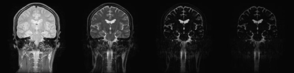
Fig 1
Acquired multi-TE images. Images were acquired by a CPMG imaging sequence with echo interval of 40 msec, echo train length of 25, with T2 ranging from 40 msec to 1000 msec. TE value of shown images are: 40, 120, 400, and 1000 msec, from left to right.
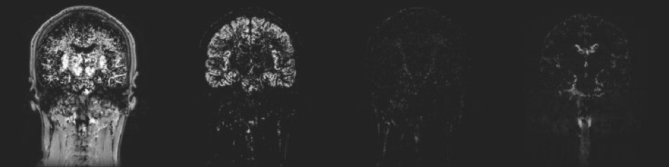
Fig 2
Result of T2 decomposition. Images acquired by CPMG sequence were decomposed into 25 T2 components, ranging from 60 msec to 2000 msec. T2 values of shown images are: 60, 80, 144 and 2000 msec, from left to right.
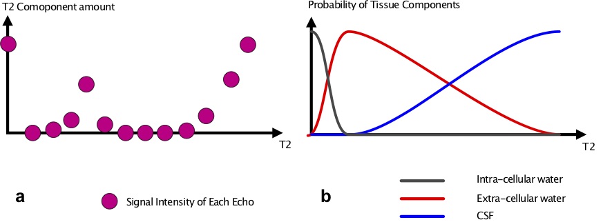
Fig 3
Amount of each T2 component are illustrated on fig 3a. By multiplying these numbers with the probability density function, amount of intra-cellular and extra-cellular water, and CSF were calculated.
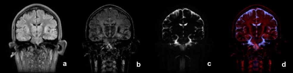
Fig 4
Result of above classification. The three components and the color map are shown: a)intra-cellular water, b) extra-cellular water, c) CSF, d) the color map.
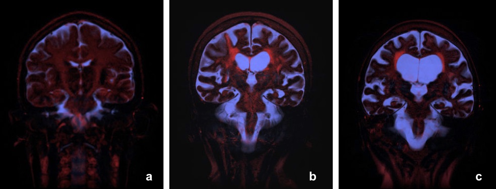
Fig 5
Typical clinical results. a) Healthy volunteer, b) Alzheimer patient 1, c) Alzheimer patient 2.