Introduction

Various electrical properties tomography (EPT) methods have been developed, which noninvasively reconstruct conductivity and permittivity maps in a human body given a radio-frequency magnetic field ($$$H^+:=(H_x+iH_y)/2$$$)¹. We proposed a new iterative EPT method based on Helmholtz decomposition of the electric field at ISMRM 2021². Our previous method can reliably reconstruct 3D EPs, and its convergence is theoretically guaranteed. However, reconstruction errors occur due to the assumption that unmeasurable components of the magnetic field, $$$H^-(:=(H_x-iH_y)/2)$$$ and $$$H_z$$$, are zero. In this paper, we describe an extension of this previous method to consider the unmeasurable magnetic field components. Assuming that the geometrical shape of a body can be obtained via MRI, we create a homogeneous simulation model that has homogeneous EPs inside the measured body shape. Using this model, we compute $$$H^-$$$ and $$$H_z$$$ numerically. We use these as approximations of the unmeasurable components of the magnetic field in our previous method.

Method

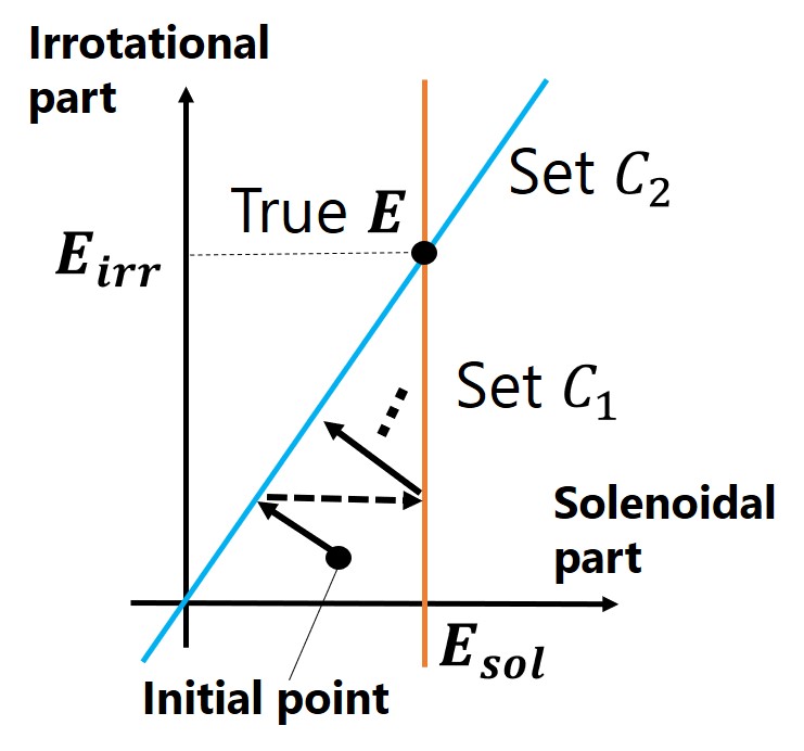
Our reconstruction algorithm² assumes that the magnetic field $$$\mathbf{H}$$$ is provided in the region of interest (ROI), $$$\Omega$$$, and the admittivity $$$\gamma:=\sigma+i\omega\epsilon$$$ is known on the boundary of $$$\Omega$$$, where $$$\sigma$$$ is the electrical conductivity and $$$\epsilon$$$ is the permittivity, and $$$\omega/2\pi$$$ is the Larmor frequency. Our algorithm starts the Helmholtz decomposition³ of a true electric field $$$\mathbf{E}$$$ in a bounded ROI given by $$$\mathbf{E}=\mathbf{E}_{irr}+\mathbf{E}_{sol}$$$, where $$$\mathbf{E}_{irr}$$$ and $$$\mathbf{E}_{sol}$$$ are the irrotational and solenoidal parts of $$$\mathbf{E}$$$, respectively, represented by \begin{align}\mathbf{E}_{irr}(\mathbf{r}')&=-\int_{\Omega}{\bigl(\mathbf{E}(\mathbf{r})\cdot\nabla\bigr)\nabla\frac{1}{4\pi|\mathbf{r}-\mathbf{r}'|}}dV,\tag{1}\\ \mathbf{E}_{sol}(\mathbf{r}')&=-\int_{\partial\Omega}\biggl(\mathbf{n}\times\frac{1}{\gamma}(\nabla\times\mathbf{H})\biggr)\times\nabla\frac{1}{4\pi|\mathbf{r}-\mathbf{r}'|}\,dS-i\omega\mu\int_{\Omega}{\mathbf{H}\times\nabla\frac{1}{4\pi|\mathbf{r}-\mathbf{r}'|}}\,dV.\tag{2}\end{align}Note that Eq. (2) is derived using Faraday's law $$$\nabla\times\mathbf{E}=-i\omega\mu\mathbf{H}$$$ and Ampere's law $$$\nabla\times\mathbf{H}=\gamma\mathbf{E}$$$. Eq. (2) shows that $$$\mathbf{E}_{sol}$$$ can be computed from the given values under the assumptions. Here, we define the following sets: \begin{align}C_1:=&\{\mathbf{f}\,|\,\mathbf{f}=\mathbf{E}_{sol}-\int_{\Omega}{\bigl(\mathbf{g}(\mathbf{r^\prime})\cdot\nabla^\prime\bigr)\nabla^\prime\frac{1}{4\pi|\mathbf{r}-\mathbf{r}'|}}dV^\prime, \,\,\hbox{where $\mathbf{g}$ is any vector field}\}, \tag{3}\\C_2:=&\{\mathbf{f}\,|\,\mathbf{f}=a\nabla\times\mathbf{H},\,\,\hbox{where $a$ is any scalar field}\}.\tag{4}\end{align} Because $$$\mathbf{E}\in C_1\cap C_2$$$, our algorithm estimates the element of $$$C_1\cap C_2$$$ by alternating the orthogonal projections⁴ schematically represented in Figure 1. After estimating $$$\mathbf{E}$$$, $$$\gamma$$$ is determined as $$$\gamma=\frac{|\nabla\times\mathbf{H}|^2}{\mathbf{E}\cdot(\nabla\times\mathbf{H})^*}$$$ from Ampere's law. This is our previous method.
Here, in the algorithm, we need to compute $$$\mathbf{H}$$$ and $$$\nabla\times\mathbf{H}$$$ given by \begin{align}\mathbf{H}&=\begin{bmatrix}H^++H^-\\-i(H^+-H^-)\\H_z\end{bmatrix},\nabla\times\mathbf{H}=\begin{bmatrix}\partial_yH_z+i\partial_z(H^+-H^-)\\ \partial_z(H^++H^-)-\partial_xH_z\\-4i\partial H^+-i\partial_zH_z\end{bmatrix},\tag{5}\end{align} with $$$\partial:=(\partial_x-i\partial_y)/2$$$. A problem with our previous method is that the unmeasurable components $$$H^-$$$ and $$$H_z$$$ are set to zero, which is a source of error. To resolve this problem, we propose to approximate the unmeasurable components with numerical simulations. Assuming that the geometry of the target body can be measured by MRI, we created homogeneous simulation models with the measured geometry and homogeneous EPs, as shown in Figure 2. Then, we simulated the magnetic field in the model using the finite element method (FEM), denoted by $$$\mathbf{H}_{hom}$$$. Finally, we approximate $$$\mathbf{H}$$$ and $$$\nabla\times\mathbf{H}$$$ by substituting the unmeasurable components of the simulated $$$\mathbf{H}_{hom}$$$, denoted by $$$H^-_{hom}(:=(H_{x,hom}-iH_{y,hom})/2)$$$ and $$$H_{z,hom}$$$, into those of the true $$$\mathbf{H}$$$, which is given by \begin{align}\mathbf{H}&\simeq\begin{bmatrix}H^++H^-_{hom}\\-i(H^+-H^-_{hom})\\H_{z, hom}\end{bmatrix},\nabla\times\mathbf{H}\simeq\begin{bmatrix}\partial_yH_z+i\partial_z(H^+- H^-_{hom})\\ \partial_z(H^++H^-_{hom})-\partial_xH_{z,hom}\\-4i\partial H^+-i\partial_zH_{z,hom}\end{bmatrix}.\tag{6}\end{align} The proposed method determines $$$C_1$$$ and $$$C_2$$$ from $$$\mathbf{H}$$$ and $$$\nabla\times\mathbf{H}$$$ in Eq. (6) and then reconstructs the EPs using our previous method.

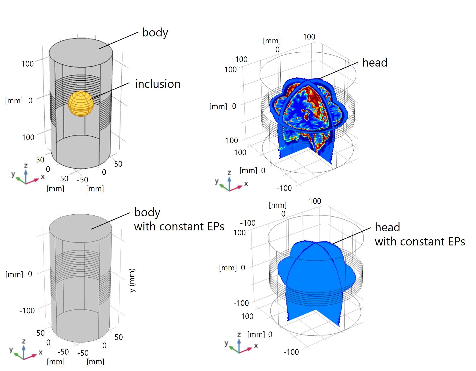
We verified our method using numerical simulations. In the simulations, the magnetic field data were computed using FEM software (COMSOL Multiphysics, COMSOL Inc.). Two simulation phantoms were modeled. As shown in Fig. 2, Model 1 was a simple model with a sphere (radius $$$=30$$$ mm, $$$\sigma=1.0$$$ S/m, $$$\epsilon_r= 50$$$) inside a cylinder representing a body (radius $$$=72$$$ mm, height $$$=270$$$ mm, $$$\sigma=0.5$$$ S/m, $$$\epsilon_r=80$$$). Model 2 was a head model simplified from the Aubert-Broche's model⁵ by reducing the number of tissue types to five: cerebral-spinal fluid, white matter, gray matter, skull, and scalp. The EPs of the homogeneous models for Model 1 and Model 2 were set to be those of the body and the means of the true EPs in a whole brain ($$$\sigma=0.62$$$ S/m, $$$\epsilon_r=59$$$), respectively. We reconstructed the EPs using the proposed method and our previous method² with the true EPs on the boundary.

Results and Discussion

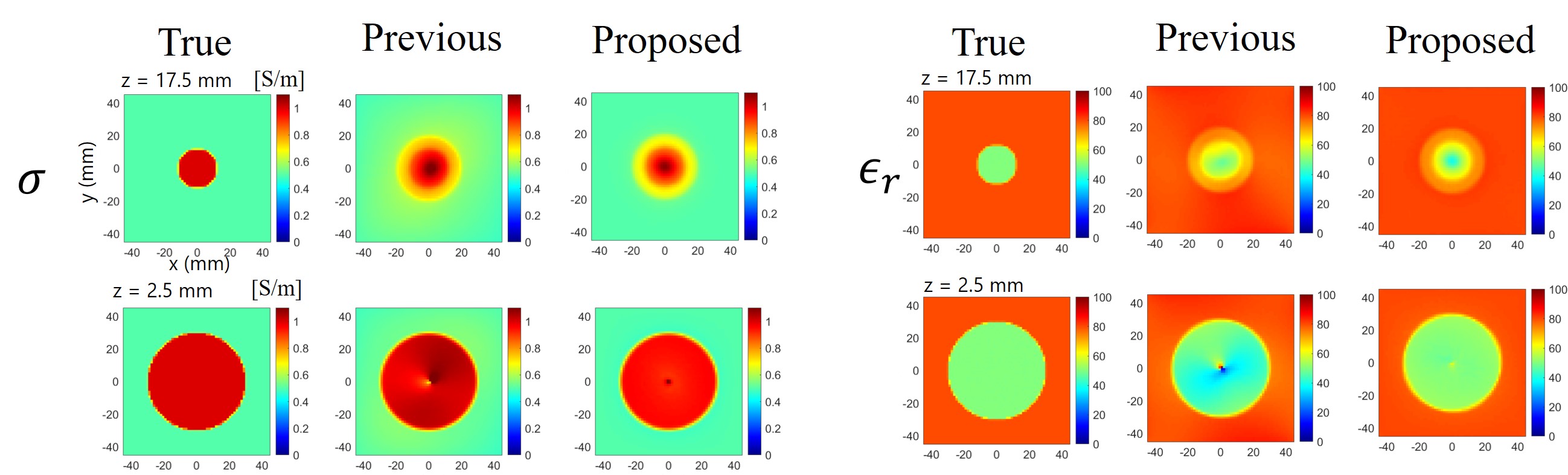
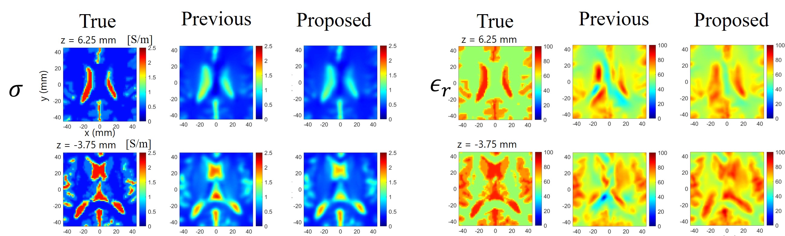
The proposed method outperformed the previous method with Model 1 (Figure 3), especially in the background region. Also, it was observed that the proposed method can suppress the spot-like artifact at the center of the slice. Although this artifact was caused by the ill-posedness of the equation $$$\gamma=\frac{|\nabla\times\mathbf{H}|^2}{\mathbf{E}\cdot(\nabla\times\mathbf{H})^*}$$$ at the center because $$$E_z$$$ is close to zero, the proposed method can reconstruct $$$\gamma$$$ better at the center because $$$E_x$$$ and $$$E_y$$$ whose amplitudes are small but relatively greater than that of $$$E_z$$$ are accurately estimated by consideration of all $$$\mathbf{H}$$$ even if $$$E_z$$$ is close to zero. In Model 2, the proposed method can reconstruct the permittivity values with greater accuracy (Figure 4) due to the suppression of artifacts as in Model 1.

Conclusion

In this study, we extended our previous method by approximating unmeasurable magnetic field components using a homogeneous model that has homogeneous EPs in a measured body shape. The method was verified by numerical simulations. The results showed that the proposed method can suppress artifacts even if the target has complicated 3D EPs, as in a brain.

Acknowledgements

This work was financially supported by Canon Medical Systems Corporation.