3218
Development of self-calibrating B1 correction for three-dimensional variable flip angle T1 mapping
Nagomi Fukuda1, Yuki Kanazawa2, Hiroaki Hayashi3, Yuki Matsumoto2, Masafumi Harada2, Motoharu Sasaki2, and Akihiro Haga2
1Institute of Biomedical Sciences, Tokushima University Graduate School, Tokushima, Japan, 2Graduate school of Health Science, Tokushima University, Tokushima, Japan, 3Faculty of Health Sciences, Institute of Medical, Pharmaceutical and Health Sciences, Kanazawa University, Kanazawa, Japan
1Institute of Biomedical Sciences, Tokushima University Graduate School, Tokushima, Japan, 2Graduate school of Health Science, Tokushima University, Tokushima, Japan, 3Faculty of Health Sciences, Institute of Medical, Pharmaceutical and Health Sciences, Kanazawa University, Kanazawa, Japan
Synopsis
We determine the accuracy of our B1 correction method using a cylindrical digital phantom and a digital brain phantom. Comparing the B1 correction accuracy of each sample, the relative uncertainties of each T1 value were less than 5%, and when long TR, the accuracy of B1 correction was almost equal to short TR. In addition, our method enabled us to correct the slice direction accurately. The proposed method can correct B1 inhomogeneity with high accuracy to in-plane and slice direction without additional scanning
Introduction
The variable flip angle (VFA) T1 mapping with a spoiled gradient-echo (SPGR), though it has a shorter scanning time than the inversion recovery method, is affected by B1 inhomogeneity caused by a transmitted radiofrequency pulse. In this situation, B1 inhomogeneity correction is required for accurate T1 estimation. The typical methods of B1 correction, are Bloch-Siegert shift, double flip angle (DFA), and actual flip angle methods. On the other hand, these methods need additional scanning for B1 mapping, except the main scan for T1 estimation; these methods require a longer total scan time. In this study, we developed a self-calibrating B1 correction method based on the DFA technique without additional scanning. The purpose of this study is to determine the accuracy of the B1 correction in our developed method using a cylindrical digital phantom and a digital brain phantom.Methods
In this study, data acquisition was used a Bloch simulator (MRIsimulations Inc.). Figure 1 shows a schematic diagram of self-calibrating B1 correction for VFA T1 mapping in this study. Built-in VFA datasets for cylindrical phantom and brain phantom were acquired using a three-dimensional spoiled gradient-echo (3D-SPGR) sequence. Table 1 summarizes relaxation times of each sample in the built-in a numerical phantom. A cylindrical phantom consisted of nine tubes having different relaxation times; T1 range, 367-1616 ms; T2 range, 32-110 ms. The digital brain phantom we used was a Colin 27 Average Brain (http://www.bic.mni.mcgill.ca//ServicesAtlases/Colin27Highres). The SPGR signal $$$S_{SPGR}$$$ is described as follows:$$S_{SPGR} = M_{0}\sin(\alpha)\frac{1-\exp(-\frac{TR}{T_{1}})}{1-\exp(-\frac{TR}{T_{1}})\cos(\alpha)}, (Eq. 1)$$
where $$$M_{0}$$$ is the equilibrium magnetization, $$$\alpha$$$ is flip angle (FA), and TR is repetition time (TR). In this study, the imaging parameters were TR = 10 and 100 ms, echo time (TE) = 4 ms, FA = 2-16 and 5-70 degrees (8 point, respectively), and matrix size = 256×256×256. After acquiring each VFA dataset, B1 inhomogeneity distribution was generated in the in-plane and slice direction using a Gaussian distribution. B1 inhomogeneity distribution was applied to each SPGR image. Next, DFA function $$$B_{1,DFA}^{function}$$$ was defined with DFA method and Gaussian distribution as follows:
$$B_{1,DFA}^{function} = \arccos(\frac{S_{2\alpha}}{2S_{\alpha}})\times{A}\times\left[-\frac{(x-\mu)^{2}}{2\sigma_x^2}-\frac{(y-\mu)^{2}}{2\sigma_y^2}-\frac{(z-\mu)^{2}}{2\sigma_z^2}\right], (Eq. 2)$$
where $$${A}$$$ is coefficient, $$$\sigma$$$ is standard deviation, and $$$\mu$$$ is mean. To generate DFA function, Eq. 1 and 2 were used and the simulation parameters were set to $$$M_{0}$$$ =1000, TR = 10 and 100 ms, FA = 15,30 and 30, 60 degrees, T1 = 300-3500, A = 0.8, $$$\mu$$$ = 0.5, and $$$\sigma_{x,y,z}$$$ = 0.5-1.0. Finally, the T1 measurement was applied to SPGR dataset of different FAs by linear least squares approximation as follows:
$$\left(\begin{array}{c}\frac{S_{1}}{\sin(B_{1,DFA}^{function}\times{\alpha_{1})}}\\\frac{S_{2}}{\sin(B_{1,DFA}^{function}\times{\alpha_{2})}}\\\ \vdots\\ \frac{S_{n}}{\sin(B_{1,DFA}^{function}\times{\alpha_{n})}}\end{array}\right)=\begin{pmatrix}\frac{S_{1}}{\tan(B_{1,DFA}^{function}\times{\alpha_{1}})} & 1 \\\frac{S_{2}}{\tan(B_{1,DFA}^{function}\times{\alpha_{2}})} &1 \\\vdots &\vdots \\\frac{S_{n}}{\tan(B_{1,DFA}^{function}\times{\alpha_{n}})} &1 \\\end{pmatrix}\cdot\left(\begin{array}{c}\exp(-\frac{TR}{T_{1}})\\ M_{0}(1-\exp(-\frac{TR}{T_{1}}))\end{array}\right), (Eq. 3)$$
In the experiment using the cylindrical phantom, T1 measurements were evaluated in each region in the in-plane and slice direction. Then, the relative uncertainties for the original and with T1 applied to B1 correction were calculated for each sample. For the brain phantom experiment, the brain segmentation was performed using statistical parametric mapping software which was divided into white matter (WM), gray matter (GM) and cerebrospinal fluid (CSF). The mean T1 values were measured at each segmented region. Additionally, the relative uncertainties map between original and T1 applied to B1 correction were calculated and the in-plane and slice direction were evaluated.
Results & Discussion
Figure 2 shows the results of calculated T1 maps and the graphs for the relationship between T1 value and the relative uncertainties found in the cylindrical phantom. Figure 3 shows the relationship between T1 values in eight samples and slice position on the cylindrical phantom. Figure 4 shows the relative uncertainties map with and without B1 correction in each region of the brain phantom. The yellow images show the masked region of each brain component. In the cylindrical phantom experiment, comparing the B1 correction accuracy of each sample in-plane, the relative error of each T1 value was found to be less than 5%. These results indicate that there is sufficient correction accuracy. In addition, the relative error values of long T1 samples were smaller than that of short T1 samples. When there is a long TR, the accuracy of B1 correction was almost equal to short TR (Fig. 3). This enabled us to accurately corrected for the slice direction at No.7 sample. On the other hand, for the No.8 sample, there were increasing T1 values at the end-slice positions (Fig. 3, red arrows). We demonstrated that our B1 correction method was successful without additional scanning. In this experiment, although T1 values were calculated using eight-data points, some data points remain a matter of research: the use of a fewer data points leads to the accomplishment of shorter acquisition times. In the future, the accuracy of our B1 correction method needs to be more investigated using fewer data points.Conclusion
It was found that our self-calibrating B1 correction method has high accuracy for in-plane and slice direction. Our B1 correction method makes it possible to calculate a 3D-T1 map using VFA method of the brain without additional scanning.Acknowledgements
No acknowledgement found.References
- Sacolick LI, Wiesinger F, Hancu I, Vogel MW. B1 mapping by Bloch-Siegert shift. Magn Reson Med. 2010 ;63(5):1315-22.
- Yarnykh VL. Actual flip-angle imaging in the pulsed steady state: a method for rapid three-dimensional mapping of the transmitted radiofrequency field. Magn Reson Med. 2007 ;57(1):192-200.
- Liberman G, Louzoun Y, Ben Bashat D. T₁ mapping using variable flip angle SPGR data with flip angle correction. J Magn Reson Imaging. 2014 ;40(1):171-80.
- Siversson C, Tiderius CJ, Dahlberg L, Svensson J. Local flip angle correction for improved volume T1-quantification in three-dimensional dGEMRIC using the Look-Locker technique. J Magn Reson Imaging. 2009 ;30(4):834-41.
- Nehrke K, Börnert P. DREAM--a novel approach for robust, ultrafast, multislice B₁ mapping. Magn Reson Med. 2012 ;68(5):1517-26
Figures
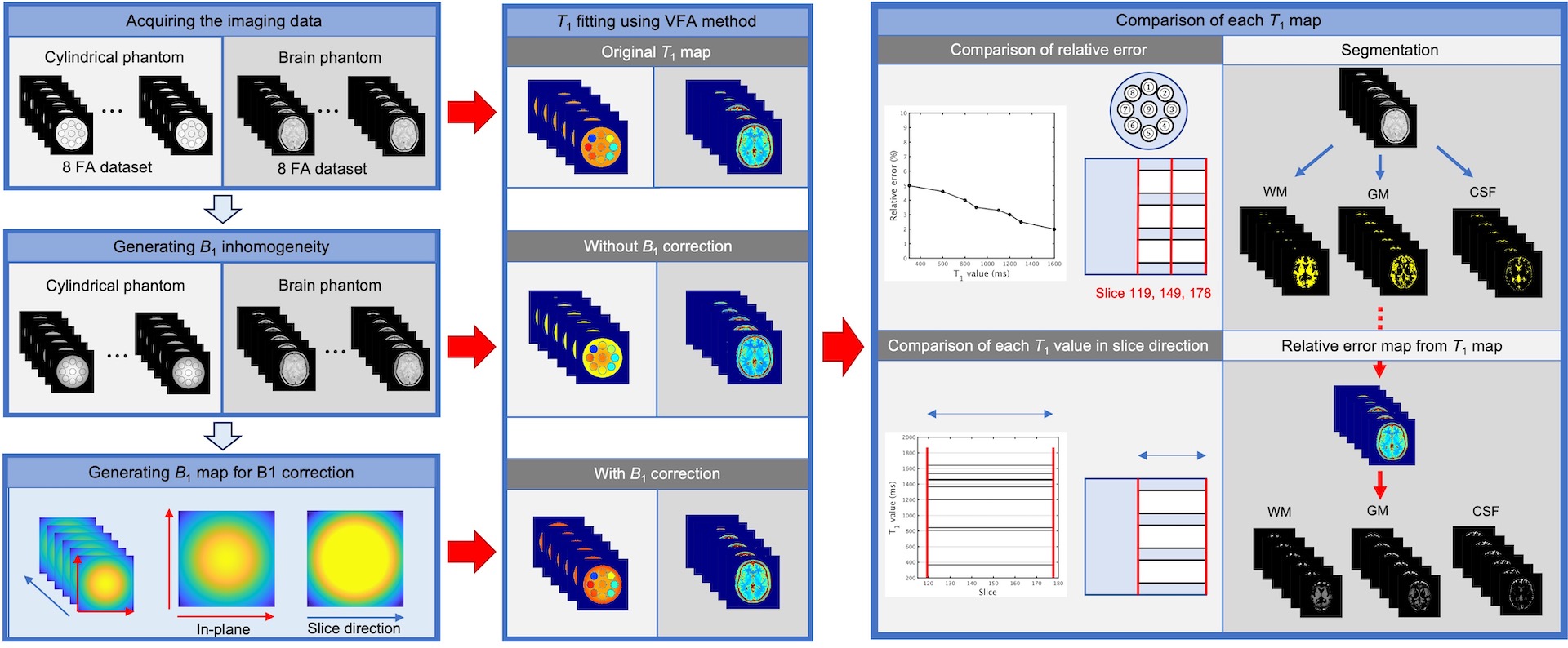
Figure 1 A schematic diagram of self-calibrating B1 correction for VFA T1 mapping.
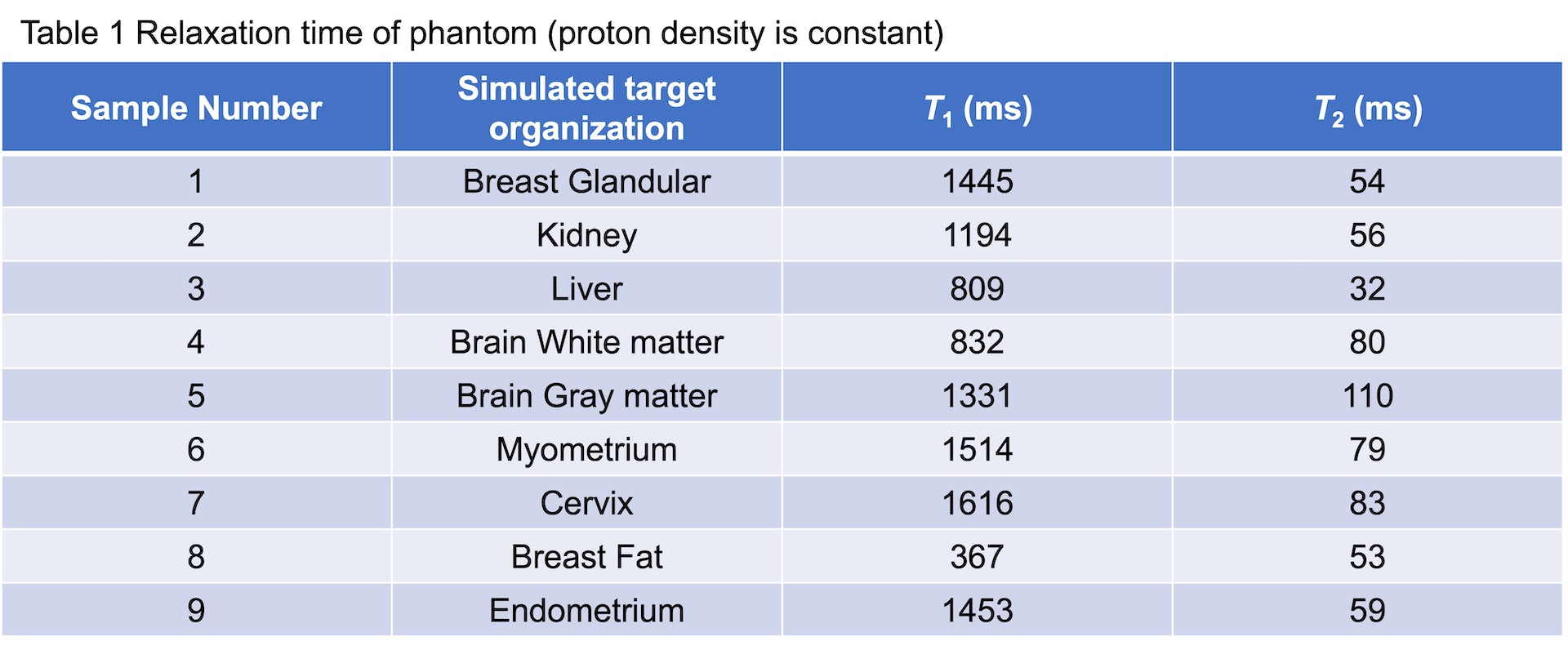
Table 1 Relaxation time of each sample in the built-in a numerical phantom.
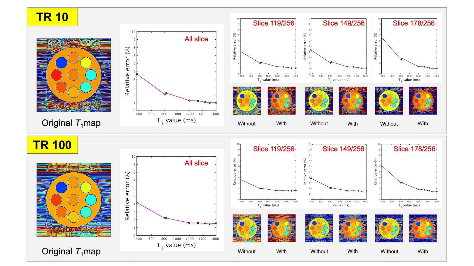
Figure 2 The measured T1 maps with and without B1 correction and the graphs for the relationship between T1 value and the relative uncertainties in the cylindrical phantom. Upper low show T1 measurement calculated from TR = 10 ms dataset, lower from TR = 100 ms.
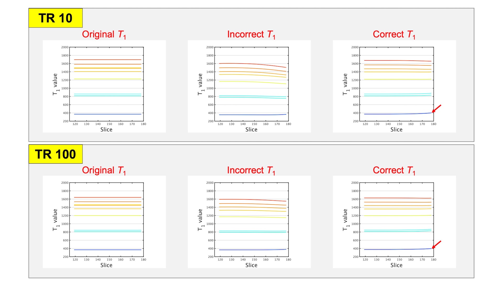
Figure 3 The relationship between T1 values in eight samples and slice position on the cylindrical phantom. Left show original T1 values, middle incorrect, right correct. Upper low show T1 measurement calculated from TR = 10 ms dataset, lower from TR = 100 ms.
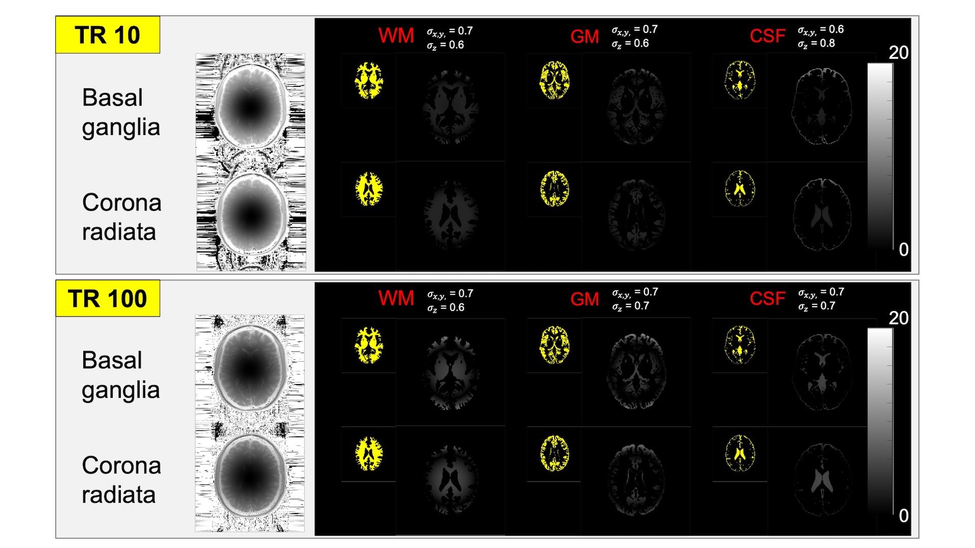
Figure 4 The relative uncertainties map with and without B1 correction in WM, GM, and CSF region of the brain phantom. Slice section are basal ganglia and corona radiata.
DOI: https://doi.org/10.58530/2022/3218