3187
Real-time Reconstruction for Accelerated MR Thermometry Using CRNN in MRgLITT Treatment
Ziyi Pan1, Jieying Zhang1, Kai Zhang2, Hao Sun3, Meng Han3, Yawei Kuang3, Jiaqi Dou1, Wenbo Liu3, and Hua Guo1
1Center for Biomedical Imaging Research, Department of Biomedical Engineering, School of Medicine, Tsinghua University, Beijing, China, 2Beijing Tiantan Hospital, Capital Medical University, Beijing, China, 3Sinovation Medical, Beijing, China
1Center for Biomedical Imaging Research, Department of Biomedical Engineering, School of Medicine, Tsinghua University, Beijing, China, 2Beijing Tiantan Hospital, Capital Medical University, Beijing, China, 3Sinovation Medical, Beijing, China
Synopsis
MRI-guided laser-interstitial thermal therapy (MRgLITT) is a minimally invasive therapeutic method in neurosurgery. Accelerating the data acquisition of thermometry for MRgLITT treatment is crucial in achieving high temporal-spatial resolution and large volume coverage. In this work, we suggest using the convolutional recurrent neural network (CRNN) to achieve real-time reconstruction for accelerated temperature mapping, because CRNN is capable of utilizing the temporal correlations of dynamic data to resolve aliasing artifacts. Results demonstrate that 6-fold acceleration can be achieved in MRgLITT treatment using CRNN with clinically acceptable reconstruction time and temperature measurement errors.
Introduction
MRI-guide laser-interstitial thermal therapy (MRgLITT) is a promising technique that can treat multiple diseases. Temperature imaging based on proton resonance frequency (PRF) shift thermometry 1 is crucial in ensuring the safety and efficacy of LITT treatment. Acquisition acceleration is desirable in MRgLITT to achieve high temporal-spatial resolution and large volume coverage 2. Advanced acceleration techniques (e.g., compressed sensing 3) enable high acceleration factors, but the iterative reconstructions are often time-consuming 4.This study aims to reconstruct undersampled real-time PRF temperature data with low latency using deep learning. A convolutional recurrent neural network (CRNN 5) is adapted in this work to jointly exploit the spatio-temporal dependencies and the consistency over iterations to improve the reconstruction performance. The purpose of this study is to evaluate the feasibility of using CRNN-based image reconstruction for accelerated MR thermometry in MRgLITT.
Theory and Methods
Reconstruction Utilizing Spatio-temporal DependenciesThe reconstruction problem of under-sampled k-space data can be formulated as:
$$x=\operatorname{argmin} R(x)+\lambda\left\|F_{u} x-y\right\|_{2}^{2}, (1)$$
where x and y represent the series of reconstructed images and under-sampled k-space data. Fu is an under-sampling Fourier operator. R is the regularization term, and λ adjusts the weight of the data fidelity term. To introduce a CRNN block to the regularization term, an auxiliary variable z is used and the optimization process is divided into two steps.
$$z_{n+1}=\operatorname{argmin} R(z)+\mu\left\|x_{n}-z\right\|_{2}^{2}, (2)$$
$$x_{n+1}=F^{H} \Lambda F z_{n}+\frac{\lambda_{0}}{1+\lambda_{0}} F_{u}^{H} y, \Lambda_{k k}=\left\{\begin{array}{cl}1, & \text { if } k \notin \Omega \\ \frac{1}{1+\lambda_{0}} & \text {, if } k \in \Omega\end{array}\right.. (3)$$
CRNN blocks are trained to solve Eq. 2. They use recurrence over both the temporal dimension and iterations 5 to jointly exploit the spatio-temporal dependencies and the consistency over iterations. Details of the network are shown in Fig. 1. In Eq. 3, λ0=λ/μ, and Ω represents the sampled k-space points. Eq. 3 is referred to as the Data Consistency (DC) step.
Data Acquisition
Data were obtained from 10 patients with epilepsy (32.5±10.3 yo, 6 Female) who underwent MRgLITT (Sinovation Medical, MRI-Guided Laser Ablation System) treatments. All studies were approved by the local IRB. MR images were acquired on a 3T scanner (Siemens, Verio) equipped with a 16-channel coil. A GRE sequence was acquired: flip angle = 30°, TE =11.6 ms, TR = 76ms, matrix = 128×128, FOV = 230×230 mm2, slice thickness = 5mm, GRAPPA = 3, temporal resolution = 3 s/frame. The scanning time for each patient ranged from three to five minutes according to the ablative dose applied.
Network Training and Testing
The online-reconstructed channel-combined images were normalized to [0,1], then inverse-Fourier-transformed to k-space and randomly undersampled using a Cartesian mask following a zero-mean Gaussian distribution 5. The 8 lowest spatial frequencies were acquired. Because of the limited GPU memory, each series was cut into small blocks with 6 frames and 128×32 in size.
The zero-filled-reconstructed images were used as the initial guess and full-sampled images were reconstructed after N iterations. Mean squared errors were used as the loss function. The performance of CRNN was evaluated using 3-fold cross validation. Data from 7 subjects were used for training and 3 for testing. The testing process is illustrated in Fig. 2.
For comparison, a low-rank-based iterative algorithm (Ascending Threshold Low Rank Constraint, AscLR 6) was also performed. Three metrics were used to quantitively evaluate the results, including image Structural Similarity Index (SSIM), Root-Mean-Square-Error (RMSE) and error ranges between the reconstructed temperatures from acceleration and the ground truth (within the heating zone).
Thermometry Calculations
Phase differences between each frame and the baseline reference (average of first five frames) were calculated using a complex-phase subtraction procedure 1. After B0 drift correction 1, the phase difference maps were converted to temperature images using $$$\alpha=-0.01 \mathrm{ppm} /{ }^{\circ} \mathrm{C}, \Delta T=\Delta \phi /\left(\alpha \cdot \gamma B_{0} \cdot T E\right)$$$.
Results and Discussion
Reconstruction results from 6× acceleration are shown in Fig. 3, including the magnitudes (Fig. 3A) and phases (Fig. 3B) and their corresponding error maps from the two reconstruction methods at frame 37. Note that the phase error maps were calculated from complex-phase subtraction. Compared with AscLR, CRNN produces phases with fewer errors in the heating region (red arrowheads).Fig. 4A shows the corresponding temperature maps of the same data. As shown, CRNN can produce more faithful temperature measurements for accelerated MR thermometry compared with AscLR. CRNN outperforms AscLR when there are large temperature changes (Fig. 4B), which could be explained by the fact that CRNN effectively uses recurrence over both the temporal dimension and iterations for reconstruction.
The results of the quantitative metrics and the computation time of CRNN and AscLR are reported in Table 1, which indicates the superiority of CRNN over AscLR.
Conclusion
In this work, we primarily demonstrated that CRNN could be utilized to reconstruct the real-time undersampled MR temperature data without sacrificing too much temperature measurement accuracy. The network is expected to be efficient not only in the CS sampling but also in other acceleration methods 7,8. Future work will include more datasets and incorporate other models such as traditional RNN 9.Acknowledgements
No acknowledgement found.References
1. Ishihara Y, Calderon A, Watanabe H, et al. A precise and fast temperature mapping using water proton chemical shift. Magn Reson Med 1995;34(6):814-823.2. Gaur P, Grissom WA. Accelerated MRI thermometry by direct estimation of temperature from undersampled k-space data. Magn Reson Med 2015;73(5):1914-1925.
3. Lustig M, Donoho D, Pauly JM. Sparse MRI: The application of compressed sensing for rapid MR imaging. Magn Reson Med 2007;58(6):1182-1195.
4. Jaubert O, Montalt-Tordera J, Knight D, et al. Real-time deep artifact suppression using recurrent U-Nets for low-latency cardiac MRI. Magn Reson Med 2021;86(4):1904-1916.
5. Qin C, Schlemper J, Caballero J, Price AN, Hajnal JV, Rueckert D. Convolutional Recurrent Neural Networks for Dynamic MR Image Reconstruction. IEEE Trans Med Imaging 2019;38(1):280-290.
6. Wang F, Dong Z, Chen S, et al. Fast temperature estimation from undersampled k-space with fully-sampled center for MR guided microwave ablation. Magn Reson Imaging 2016;34(8):1171-1180.
7. Han Y, Mun C. Evaluation of the keyhole technique applied to the proton resonance frequency method for magnetic resonance temperature imaging. J Magn Reson Imaging 2011;34(5):1231-1239.
8. Pruessmann KP, Weiger M, Scheidegger MB, Boesiger P. SENSE: sensitivity encoding for fast MRI. Magn Reson Med 1999;42(5):952-962.
9. Hosseini SAH, Yaman B, Moeller S, Hong M, Akcakaya M. Dense Recurrent Neural Networks for Accelerated MRI: History-Cognizant Unrolling of Optimization Algorithms. IEEE J Sel Top Signal Process 2020;14(6):1280-1291.
Figures
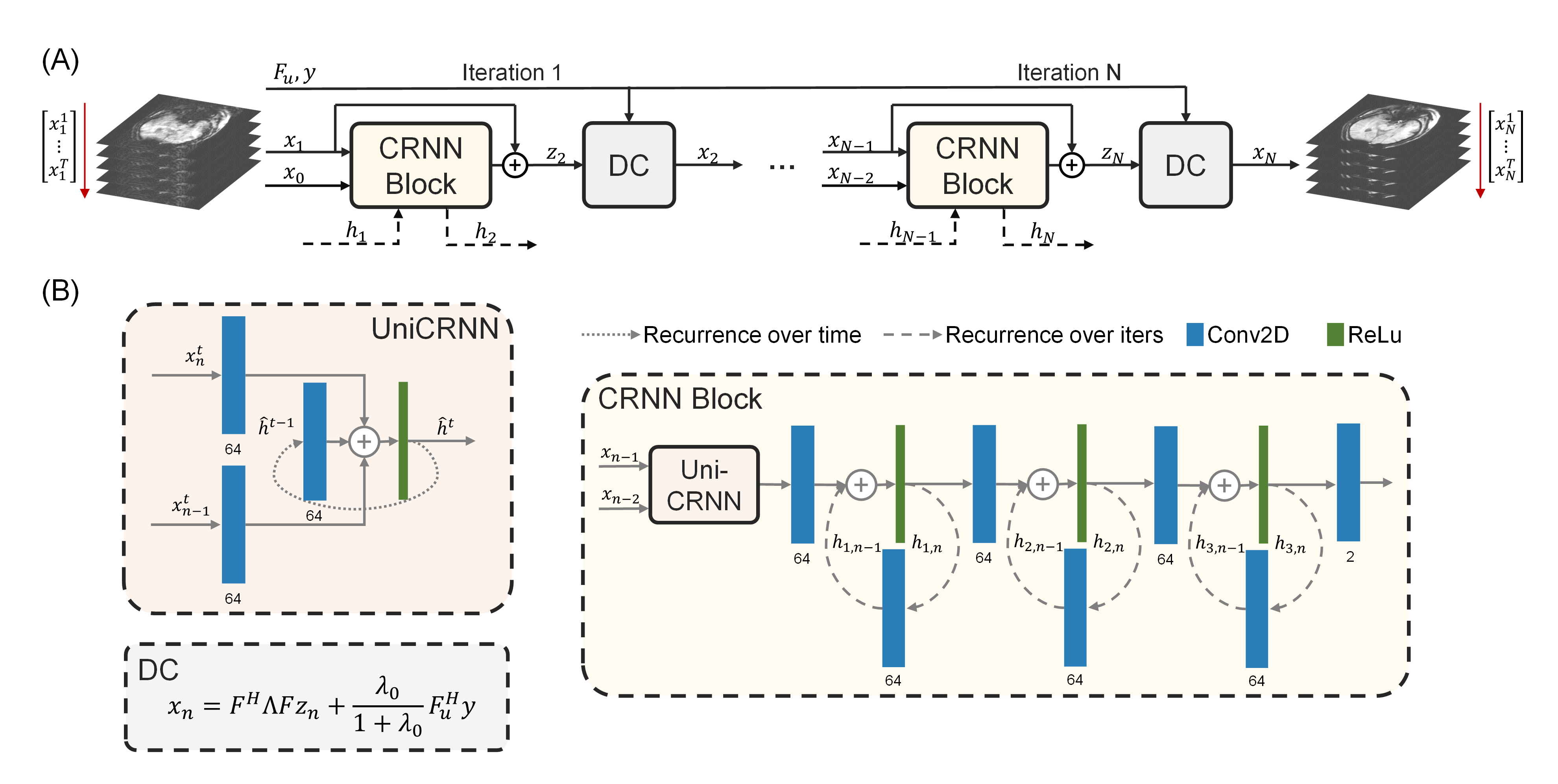
FIG. 1. CRNN for real-time MR temperature imaging. (A) The unrolled architectures of CRNN. Each iteration contains one CRNN block and one data consistency (DC) block which follows Eq. 3. (B) The first part of the CRNN block is a unidirectional convolutional recurrent unit (UniCRNN), which contains recurrence over the previous time frames and the previous iteration. It is followed by three 2D convolutional layers with ReLu activation functions, which contain recurrence over the previous iteration. The numbers of convolution kernels are marked below the layers.
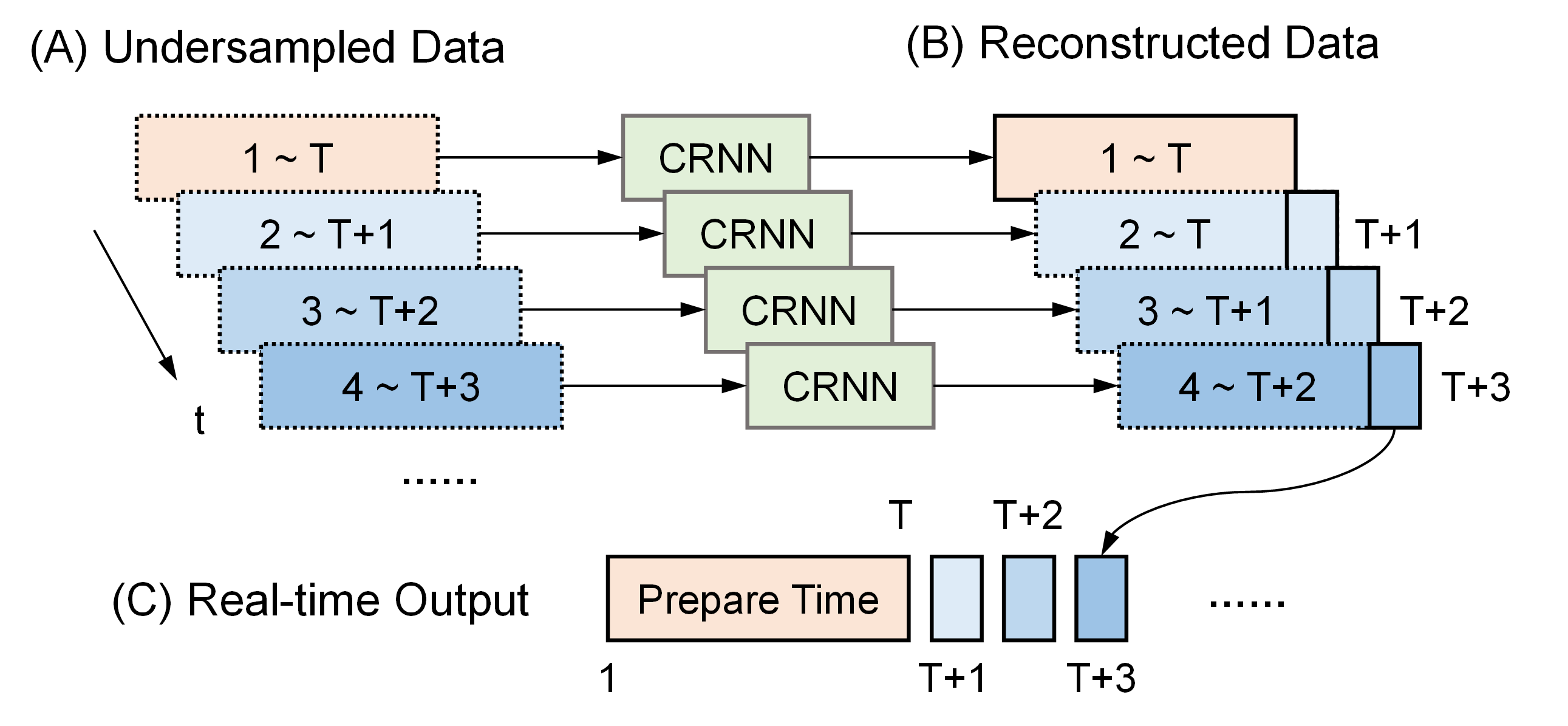
FIG. 2. A schematic diagram of real-time MRgLITT reconstruction using CRNN. The first T time frames are reconstructed simultaneously at the end of the preparation time. Real-time output is then accomplished by feeding into the CRNN network the current frame along with the previous (T-1) frames.
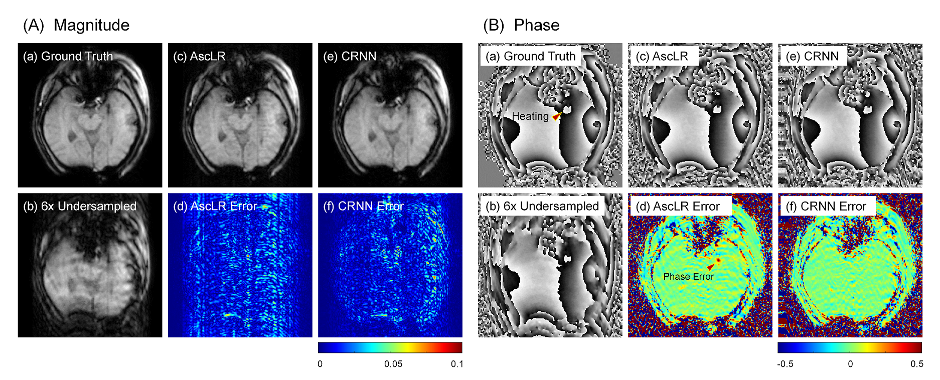
FIG. 3.
The comparison of reconstructions (A:
magnitude, B: phase) on a representative time frame with their error
maps. (a) Ground Truth, (b) Undersampled image by acceleration factor 6, (c,d)
AscLR, (e,f) CRNN.
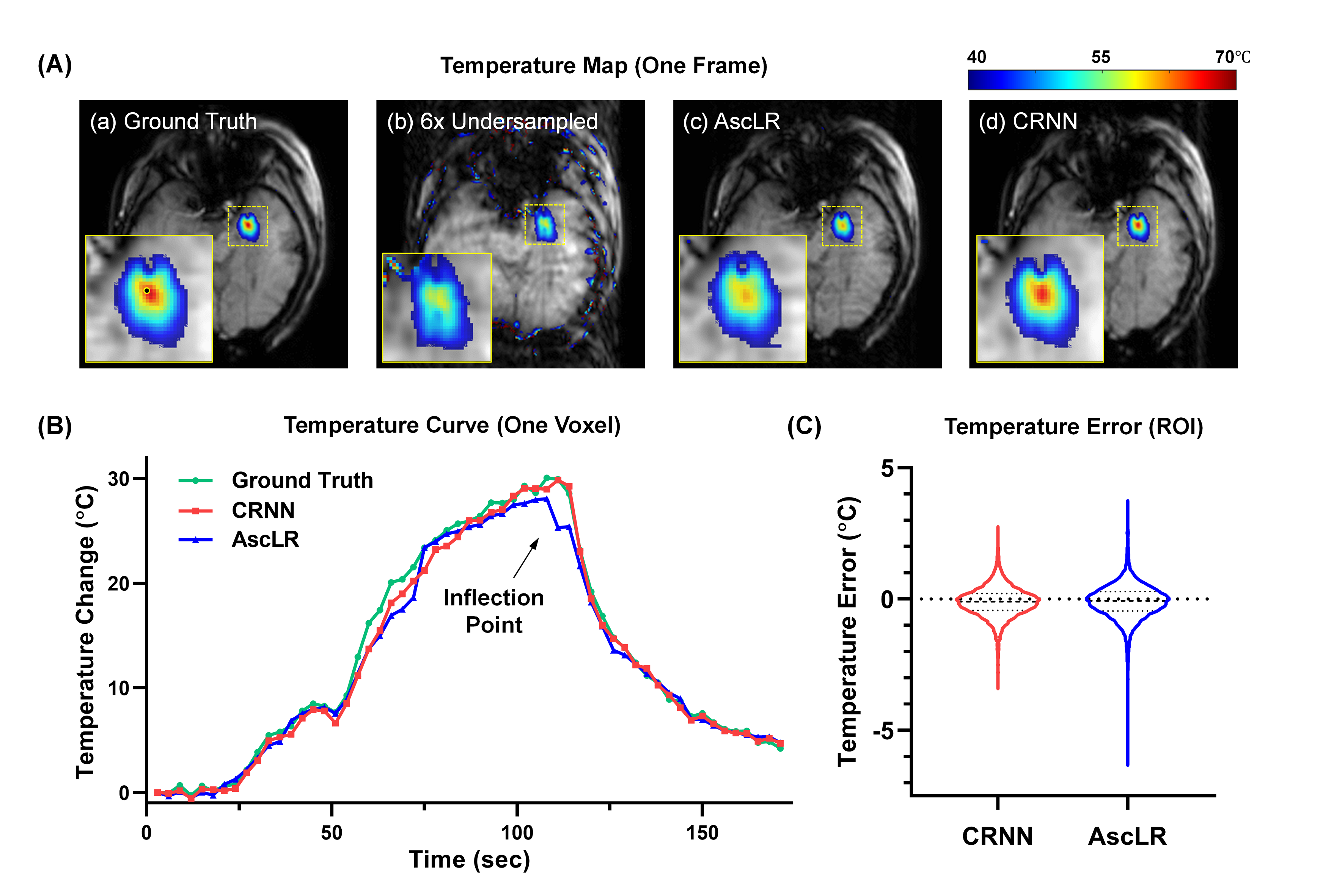
FIG. 4. The comparison of temperature measurements from the two reconstruction strategies. (A) The accelerated temperature maps calculated from (a) ground truth, (b) 6× undersampled image, (c) AscLR and (d) CRNN. (B) MRg LITT heating curves within the heating center of a representative subject. Green: ground truth; red: CRNN; blue: AscLR. (C) Temperature errors across the time frames and voxels within the heating zone.
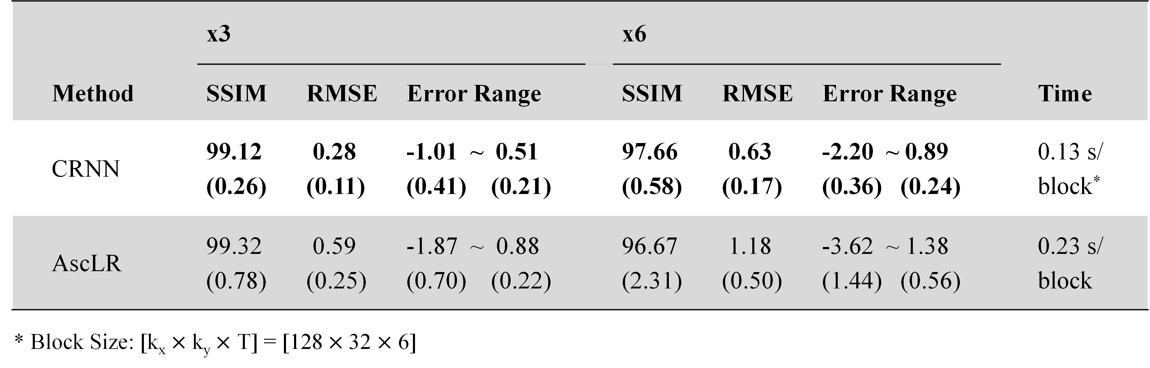
Table 1. Performance comparison (SSIM, and RMSE [℃] and Error Range [℃]) on real-time MRgLITT temperature data with different acceleration rates. Numbers shown in Table 1 are mean values of the metrics with stand deviation of different subjects in parenthesis.
DOI: https://doi.org/10.58530/2022/3187