2972
Accelerating Myelin Water Content Quantification using Deep Non-Local Sparse Model1School of Biomedical Engineering, Shanghai Jiao Tong University, Shanghai, China, 2Department of Radiology, Stanford University, Stanford, CA, United States
Synopsis
A grouping sparse coding (Group-SC) model is used in this study for the acceleration of myelin water content quantification. Images with improved quality are obtained using the Group-SC algorithm, in the aspect of minimal artefacts and good data consistency with fully-sampled labels. Myelin water fraction (MWF) maps reconstructed using Group-SC demonstrate more natural spatial distribution of myelin water in the brain. The proposed Group-SC algorithm has demonstrated its potential for the acceleration of the myelin water content quantification at R = 6.
Introduction
Myelin water imaging (MWI) can be used for the quantification of myelin water content [1]. Multi-echo T2* weighted images (T2*WIs) have been used to generate myelin water fraction (MWF) map for the whole brain, which typically takes a scan time for several minutes [2-4]. Several methods have been proposed for the acceleration of the T2*WIs [5-7], some of them have exploited the similarity information in images [6,7]. In this study, a method based on deep grouping sparse coding (Group-SC) [8] model is employed to exploit the non-local self-similarity information among patches for the quantification of myelin water content, using convolutional joint sparse coding based on a variant of LISTA algorithm [9]. The preliminary results in this study demonstrate that the acceleration of myelin water content quantification with improved image quality can be achieved using the proposed deep Group-SC method.Theory
The flowchart of the Group-SC network is illustrated in Figure 1. The Group-SC module and the data consistency module are combined in succession as a single unit, while multiple units are concatenated together. The T2*WIs are first fed to a centering operation, which means that the zero-frequency information is not processed by the model. The global self-similarity information is integrated in the model, where a $$$L_{1,2}$$$-norm is used to enforce that the group-wise sparsity is shared across similar patches. After being processed by the Group-SC module the mean value is added back, and the image as a whole will further be processed by DC module.The Group-SC and DC module in a single unit are defined as follow:
$$\min _{x, \theta} \tau\left\|Y^{C}-D A\right\|_{2}^{2}+\xi \psi(A)+\left\|F_{u} x-y\right\|_{2}^{2}\tag{1}$$
where $$$x$$$ are the desired images, $$$A$$$ represents sparse coding for a given dictionary $$$D$$$, $$$Y^{C}$$$ are the centered input patches, $$$y$$$ is the undersampled k-space data, $$$F_{u}$$$ is the undersampled Fourier operator, $$$\| \|_{2}^{2}$$$ is the Frobenius norm, and $$$\tau,\xi$$$ are the regularization parameters. $$$\psi(A)=\Lambda\|A\|_{1,2}$$$ is the group sparsity regularizer, $$$\Lambda$$$ represents different soft-thresholding parameters $$$\lambda_{i}$$$ in each inner iteration step. $$$\theta$$$ is the set of parameters to learn, including all dictionaries and the regularization parameters.
The optimization problem can then be solved by the following two consecutive steps:
$$\begin{gathered}\mathrm{B}=A_{k}+C^{T}\left(Y^{C}-D A_{k}\right), \\A_{k+1}=\max \left(1-\frac{\Lambda_{k} \sqrt{\|\Sigma\|_{1}}}{\left\|B(\Sigma)^{\frac{1}{2}}\right\|_{1,2}}, 0\right) B,\end{gathered} \tag{2}$$
where $$$C$$$ is a decoupled dictionary from $$$D$$$, and $$$\Sigma$$$ is the similarity matrix which is updated at a given frequency. The output patches are then generated using a dictionary, which is also decoupled from $$$D$$$.
Methods
Twelve healthy subjects were scanned using a multi-slice mGRE sequence on a 3T MRI scanner (uMR790, United Imaging Healthcare, Ltd., Shanghai, China). Written consent was obtained before each scan. The scanning parameters were: FOV = 240 mm × 240 mm, matrix = 176 × 176, flip angle = 90°, TR = 2 s, first TE = 1.95 ms, echo spacing = 1.16 ms, echo train length = 30, slice thickness = 3 mm, 25 slices were scanned with a 1.5 mm slice gap. The whole brain scan time was 5.9 min. A multishot variable density blipped mGRE trajectory [2] with R = 6 was used for retrospective undersampling. The data of 7 subjects were used for training, 1 subject for validation, and 4 subjects for testing. The proposed algorithm was compared to the state-of-the-art TDLLS [2] and the CRNN [10,2] algorithms. The non-negative jointly sparse (NNJS) [11] algorithm was used for MWF estimation.Results
As shown in Figure 2, results from Group-SC show good consistency with fully sampled references, which can be clearly observed from difference maps. Minimal artefacts are obtained from Group-SC reconstructed images, and the PSNR values of them are higher than that of other two algorithms. In Figure 3, the MWF maps from Group-SC outperform images from TDLLS and CRNN. The nRMSE from Group-SC are the lowest among three algorithms. Statistical results for four test subjects in Table 1 demonstrate improved performances using the proposed algorithm in comparison with other two algorithms.Discussion and Conclusion
Superior performances have been achieved using Group-SC algorithm, in the aspect of reduced artefacts and better consistency with the fully sampled references. The self-similarity information provides a powerful prior during reconstruction, which yields better reconstruction results. The Group-SC algorithm has demonstrated its potential for the acceleration of myelin water content quantification at R = 6.Acknowledgements
This study is supported by the National Key Research and Development Program (2016YFC0103905) and the National Natural Science Foundation of China (81627901).
References
[1] Laule C, Leung E, Lis DK, Traboulsee AL, Paty DW, MacKay AL, Moore GR. Myelin water imaging in multiple sclerosis: quantitative correlations with histopathology. Mult Scler. 2006;12:747-753.
[2] Chen Q, She H, Du YP. Whole Brain Myelin Water Mapping in One Minute Using Tensor Dictionary Learning With Low-Rank Plus Sparse Regularization. IEEE Trans Med Imaging. 2021;40:1253-1266.
[3] Du YP, Chu R, Hwang D, Brown MS, Kleinschmidt-DeMasters BK, Singel D, Simon JH. Fast multislice mapping of the myelin water fraction using multicompartment analysis of T2* decay at 3T: a preliminary postmortem study. Magn Reson Med. 2007;58:865-870.
[4] Lee H, Nam Y, Kim DH. Echo time-range effects on gradient-echo based myelin water fraction mapping at 3T. Magn Reson Med. 2019;81:2799-2807.
[5] Chen HS, Majumdar A, Kozlowski P. Compressed sensing CPMG with group-sparse reconstruction for myelin water imaging. Magn Reson Med. 2014;71:1166-1171.
[6] Drenthen GS, Backes WH, Aldenkamp AP, Jansen JFA. Applicability and reproducibility of 2D multi-slice GRASE myelin water fraction with varying acquisition acceleration. Neuroimage. 2019;195:333-339.[7] Chen Q, She H, Wang Z, Du YP. Global and Local Deep Dictionary Learning Network for Accelerating the Quantification of Myelin Water Content. In Proceedings of the 29th Annual Meeting of ISMRM, 2021. p. 2163.
[8] Lecouat B, Ponce J, Mairal J. Fully Trainable and Interpretable Non-local Sparse Models for Image Restoration. 2020, arXiv:1912.02456.
[9] Gregor K, LeCun Y. Learning fast approximations of sparse coding. In Proceedings of the Proceedings of the 27th ICML, 2010:399-406.
[10] Qin C, Schlemper J, Caballero J, Price AN, Hajnal JV, Rueckert D. Convolutional Recurrent Neural Networks for Dynamic MR Image Reconstruction. IEEE Trans Med Imaging. 2019;38:280-290.
[11] Chen Q, She H, Du YP. Improved quantification of myelin water fraction using joint sparsity of T2* distribution. J Magn Reson Imaging. 2020;52:146-158.
Figures
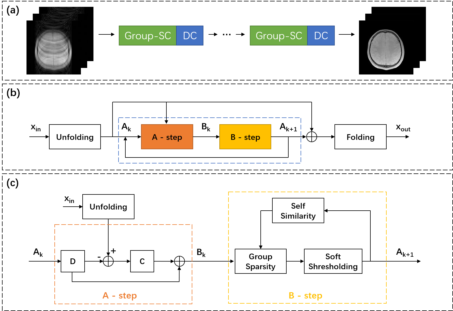

Figure 2. Comparative results of the first echo of T2*WIs in four different slices, reconstructed by TDLLS, CRNN and Group-SC algorithms with R = 6 from one subject. All difference maps are amplified 10-fold for visualization. The PSNR are showed at the bottom of each reconstructed image.
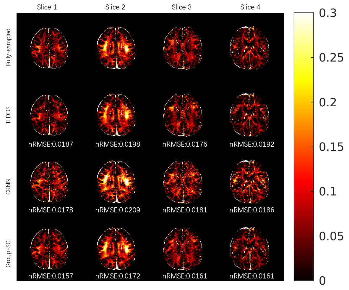
Figure 3. Comparative results for MWF map from TDLLS, CRNN and Group-SC reconstructions with R = 6 from one subject. The nRMSE are showed at the bottom of each image.
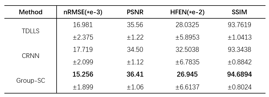
Table 1. Comparison of the statistical results from MWF maps reconstructed by TDLLS, CRNN and Group-SC algorithms of four test subjects. Four evaluations (nRMSE, PSNR, HFEN, SSIM) were calculated in terms of mean and standard deviation at R = 6.