2937
A deep learning-based background field removal method for brains containing high susceptibility sources1University of Queensland, Brisbane, Australia
Synopsis
Background field removal (BFR) is a critical step in quantitative susceptibility mapping (QSM). Eliminating the background field in brains containing high susceptibility sources, such as intracranial hemorrhages, is challenging due to the relatively large scale of the local field induced from these sources. This study proposed a new deep learning-based method, "BFRnet", and compared it with several conventional BFR methods in processing two simulated and two in vivo brain datasets. The BFRnet method was effective in background field removal for acquisitions of arbitrary orientations and performed significantly better than other methods in the regions with high susceptibility sources.
Introduction
Background Field Removal (BFR) is a critical pre-processing step of Quantitative Susceptibility Mapping (QSM) to generate local field maps without the overwhelming effect of the background field from air cavities. However, conventional BFR algorithms of iterative procedures suffer from brain edge erosion [1] and require careful parameter tuning [2, 3]. Recently, a couple of deep learning-based methods emerged [4, 5] and have demonstrated some improvements. However, these methods mainly use healthy brains as the training dataset and have not been tested on pathological brain datasets such as intracranial hemorrhage. Also, the effect of obliqueness of acquisition FOVs on background field removal requires further investigation. In this work, a new deep learning-based method, "BFRnet", is proposed to tackle these issues and is compared with another deep learning method SHARQnet [5] and three conventional BFR methods (i.e., PDF [2], LBV [3] and RESHARP [1]).Methods
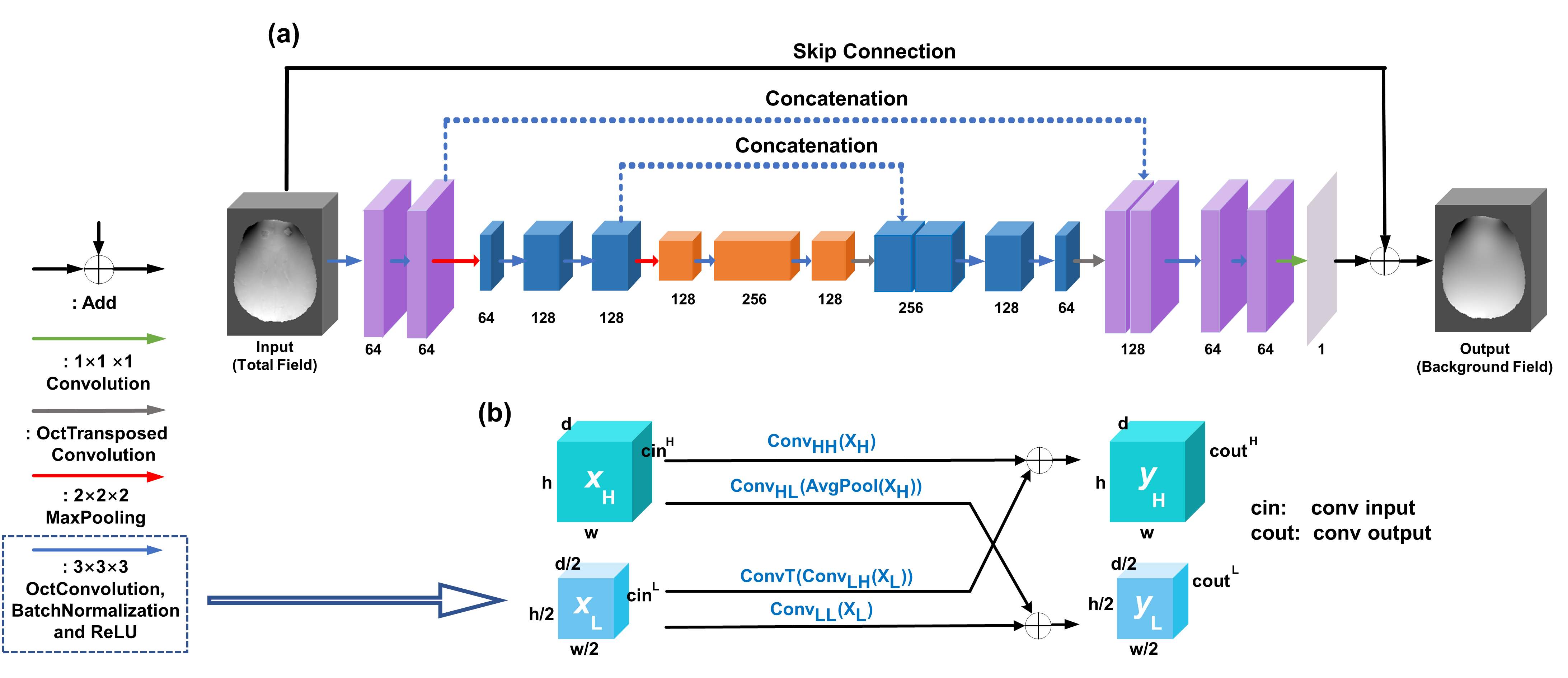
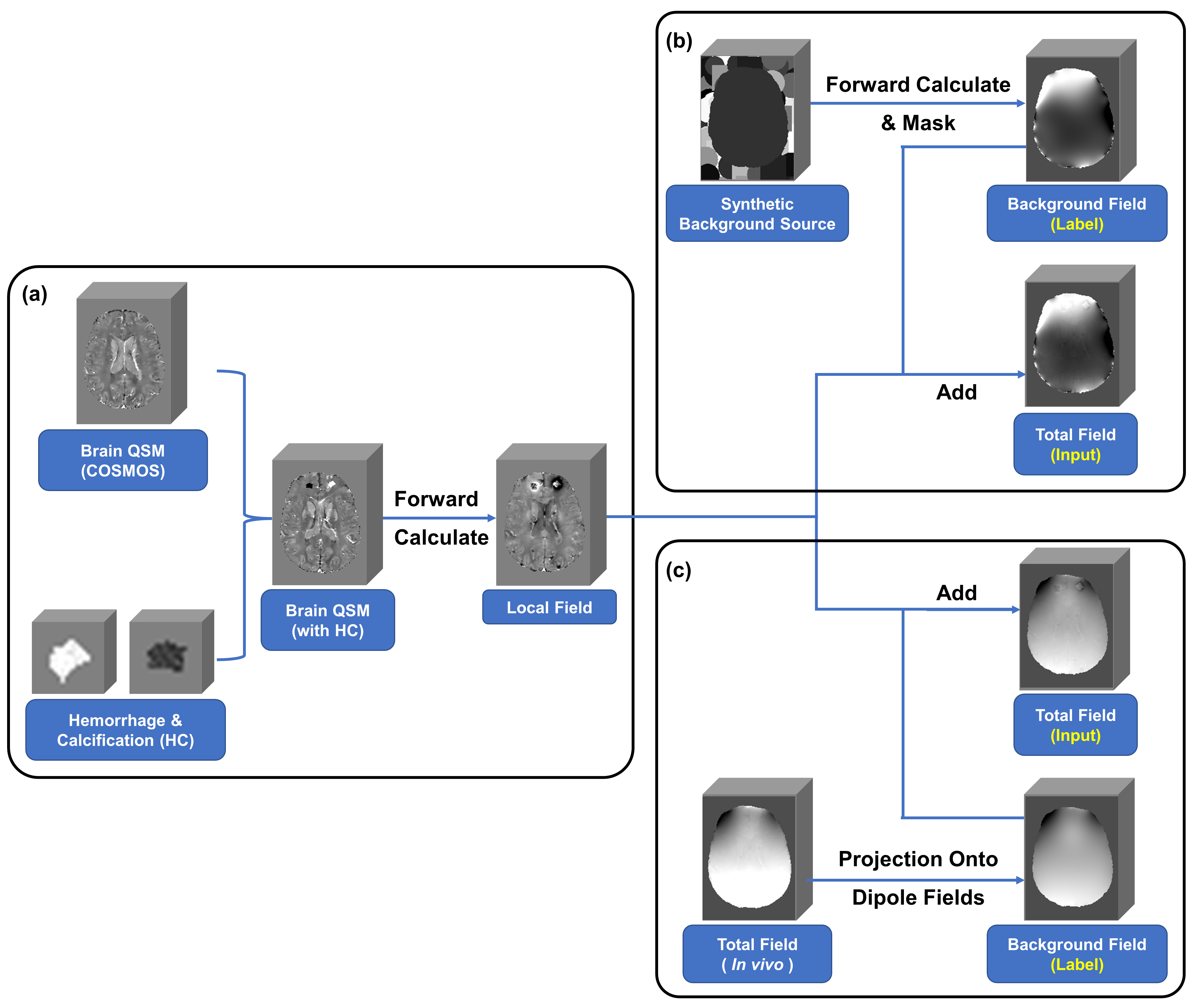
Our recently proposed Octave-network [6, 7], were used in this study. The improved neural network is referred to as "BFRnet" with network configurations of 10 (kernel size: 3×3×3) Octave convolutional layers, 2 max-pooling layers (kernel size: 2×2×2), 2 transposed Octave convolutional layers (kernel size: 2×2×2), 1 final convolutional layer (kernel size: 1×1×1), 12 batch normalization layers, and 2 feature concatenations as illustrated in Figure 1.High susceptibility sources (e.g., Hemorrhage and Calcification) were simulated and included in the training set, as shown in Figure 2(a). Two data preparation pipelines were then investigated to simulate the background field. One was generated from synthetic geometric susceptibility sources randomly distributed outside the the brain, see Figure 2(b). The other used the PDF method [2] to calculate the background field from in vivo total field map, shown in Figure 2(c). The susceptibility maps with and without simulated background sources were used to simulate the total field and local field maps, respectively. The original total field and susceptibility maps were obtained from 96 in vivo subjects (1 mm isotropic at 3T) and reconstructed using a previously developed pipeline [8]. The BFRnet was trained on 28,800 patches (matrix size: 643) cropped from the background field maps (network labels) and the total field maps (network inputs).
For simulation experiments, a COSMOS map (previously reconstructed with 1mm isotropic resolution) with added synthetic geometric background susceptibility sources was used to simulate the total field map of a healthy subject. In addition, two high susceptibility sources were superposed onto the COSMOS image to generate the pathological simulation data. Finally, for in vivo experiments, two local field maps (1 mm isotropic) were obtained by post-processing the raw phase from 2 healthy subjects at 3 T. One of them was acquired with neutral orientation (pure axial), and the other was a 15-degree angle oblique from the main field direction.
Results
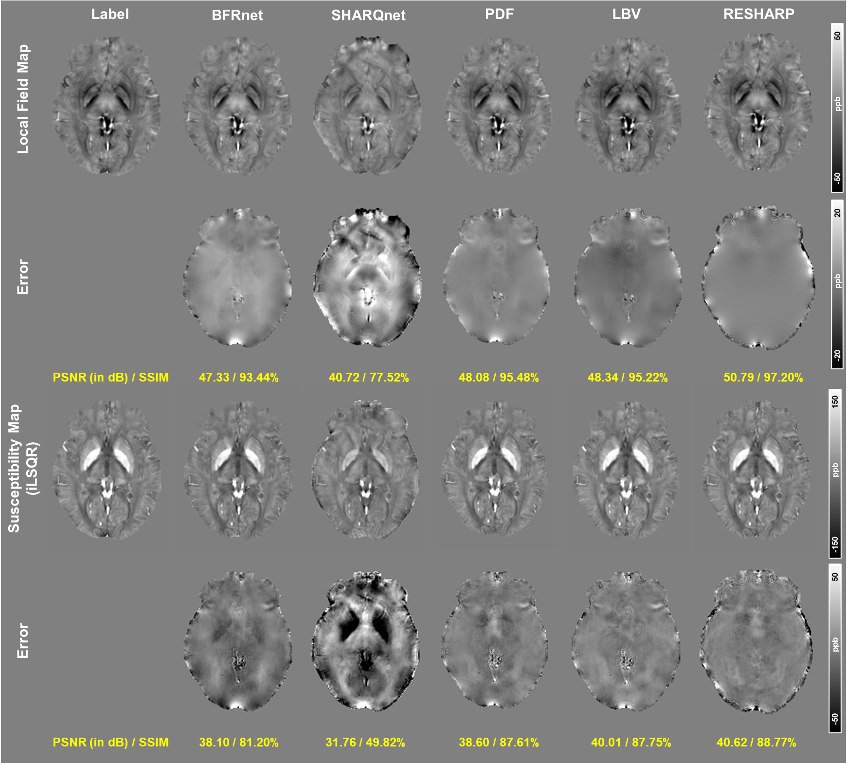
Figure 3 compares the local field results reconstructed by five methods from a total field map with the simulated synthetic background. This total field was eroded three voxels before reconstruction. The proposed BFRnet method output relatively high PSNR (47.33 dB) and SSIM (0.93), similar to conventional RESHARP, PDF and LBV methods. Substantial underestimation in the local field map was observed in the SHARQnet result. Similar trends were observed in susceptibility maps using iLSQR for dipole inversion [9].Figure 4 shows BFR results by five methods in the coronal view, containing high-susceptibility sources (e.g., hemorrhage and calcification). The BFRnet achieved similarly high PSNR (47.50 dB) and SSIM (0.94) as the RESHARP method (49.82 dB and 0.96). However, local field error maps demonstrated that the PDF, LBV and RESHARP led to significant errors in the local field induced by high-susceptibility sources. Hence, it resulted in a considerable contrast loss in the susceptibility results. The BFRnet achieved the highest susceptibility measurement among all five methods with 639.5 ppb in hemorrhage and -333.7 ppb in calcification. In contrast, PDF led to only 535.3 ppb and -310.7 ppb for hemorrhage and calcification. The reference values are 667 ppb and -342 ppb when performing iLSQR on the ground truth local field map.
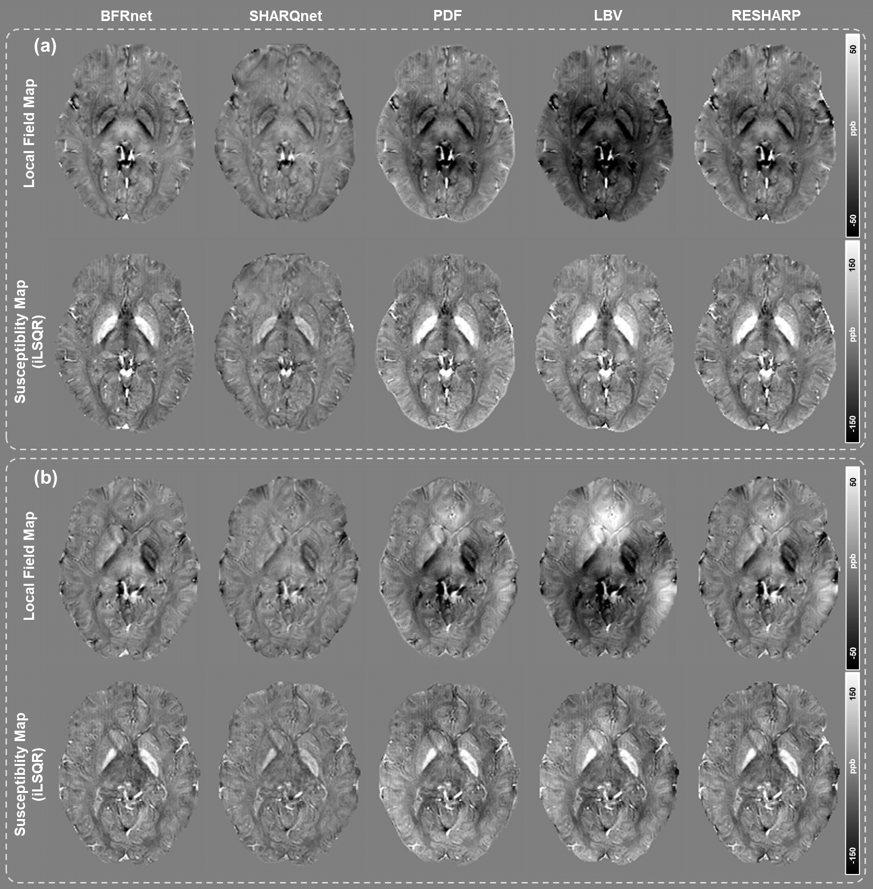
Figure 5(a) demonstrates the BFR and dipole inversion results from in vivo acquisitions with neutral orientation (i.e., pure axial acquisition). PDF and LBV results showed substantial cortex and white matter contrast loss, while BFRnet showed the best background correction among the five methods. Figure 5(b) illustrates the in vivo experiment results of BFR and iLSQR in an oblique acquisition, with FOV 15 degrees to the main field. Overall the results are similar to the neutral acquisition, where the proposed BFRnet achieved a similar result as RESHARP. While PDF and LBV showed some residual artifacts, SHARQnet significantly suppressed local field and susceptibility contrasts. The results confirm that even though the network was trained on pure-axial data acquisitions, it generalized to arbitrary head orientations.
Discussion and conclusion
A deep learning-based BFR network (BFRnet) was proposed in this study, which improved the accuracy of local field reconstruction in the hemorrhage subjects and oblique orientated scans, compared with conventional algorithms (i.e., PDF, LBV, and RESHARP) and a previous deep learning method (i.e., SHARQnet). The origin of the improvement may be due to the inclusion of high-susceptibility sources in the training process, which will be further studied.Acknowledgements
HS acknowledges support from the Australian Research Council (DE210101297).References
1. Sun, H. and A.H. Wilman, Background field removal using spherical mean value filtering and Tikhonov regularization. Magnetic resonance in medicine, 2014. 71(3): p. 1151-1157.
2. Liu, T., et al., A novel background field removal method for MRI using projection onto dipole fields. NMR in Biomedicine, 2011. 24(9): p. 1129-1136.
3. Zhou, D., et al., Background field removal by solving the Laplacian boundary value problem. NMR in Biomedicine, 2014. 27(3): p. 312-319.
4. Liu, J. and K.M. Koch. Deep Gated Convolutional Neural Network for QSM Background Field Removal. in International Conference on Medical Image Computing and Computer-Assisted Intervention. 2019. Springer.
5. Bollmann, S., et al., SHARQnet–Sophisticated harmonic artifact reduction in quantitative susceptibility mapping using a deep convolutional neural network. Zeitschrift für Medizinische Physik, 2019. 29(2): p. 139-149.
6. Gao, Y., et al., xQSM: quantitative susceptibility mapping with octave convolutional and noise‐regularized neural networks. NMR in Biomedicine, 2021. 34(3): p. e4461.
7. Zhu, X., et al., Deep grey matter quantitative susceptibility mapping from small spatial coverages using deep learning. arXiv preprint arXiv:2106.00525, 2021.
8. Sun, H., et al., Whole head quantitative susceptibility mapping using a least-norm direct dipole inversion method. NeuroImage, 2018. 179: p. 166-175.
9. Li, W., et al., A method for estimating and removing streaking artifacts in quantitative susceptibility mapping. Neuroimage, 2015. 108: p. 111-122.
Figures