2932
Investigating a residual neural network to generated customizable RF pulses for MRI1Computer Science, Mathematics, Physics, and Statistics, University of British Columbia, Kelowna, BC, Canada, 2Computer Science, Mathematics, Physics, and Statistics, University of British Columbia Okanagan, Kelowna, BC, Canada, 3Biomedical Engineering and Imaging Institute, Icahn School of Medicine at Mount Sinai, New York, NY, United States
Synopsis
We investigate a method for the design of radio frequency (RF) pulses for custom simultaneous multi slice spatial profiles. We trained a variation of residual neural networks on a dataset of 96,000 generated adiabatic “power independent of the number of slices” (PINS) RF pulses, varying parameters such as gradient duty cycle, number of pulse lobes, quadratic phase strength, and transition and filter bandwidth. We compared the direct-design RF pulses to those generated by our model.
Introduction
Simultaneous multislice (SMS) MRI can accelerate acquisition times with minimal impact on image signal to noise ratio (SNR)1,2. A Power Independent of Number of Slices (PINS) pulse design allows for the creation of SMS pulses that do not increase the overall power deposition. However, the development of a pulse to match the custom spatial parameters required of particular applications is a non-linear, time consuming process which requires iterative tuning2,3. We attempt to simplify the design process by training a residual neural network (ResNet) on a large dataset of generated RF pulses from the SEAMS PINS algorithm1. For a given spatial profile, the model output generates the RF pulse.Methods
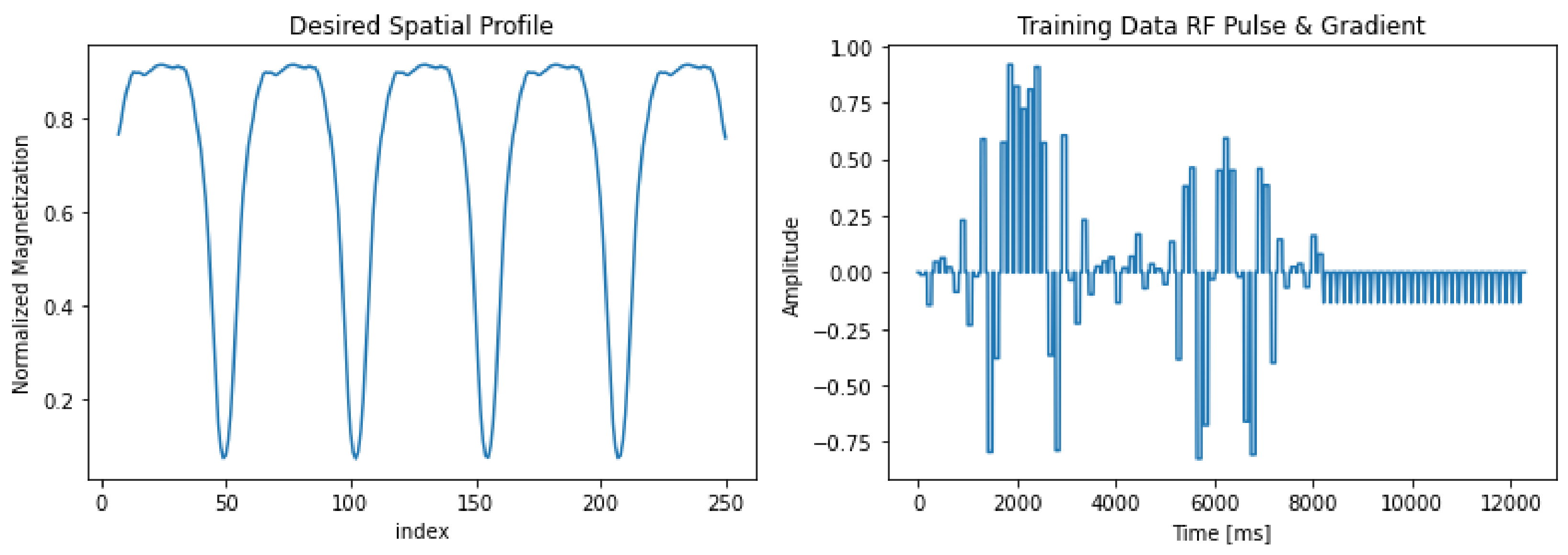
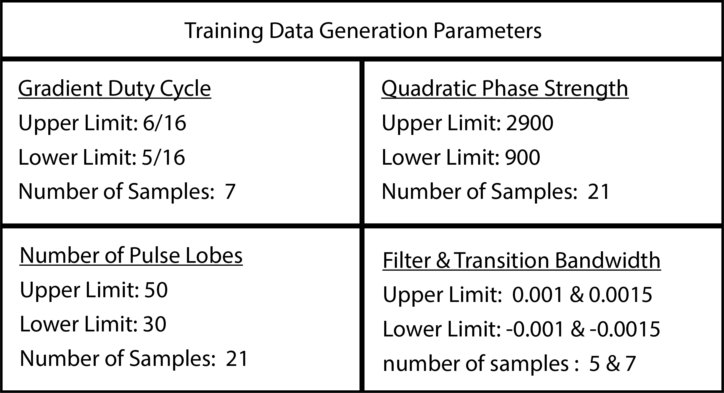
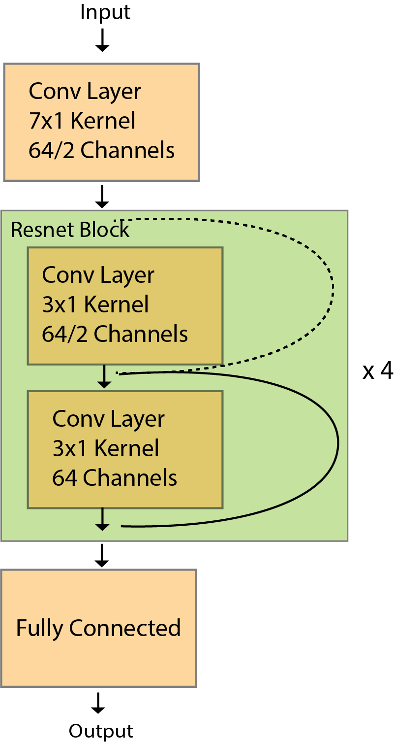
Previous work has proposed a ResNet that shows good preliminary results in deep learning simulations of Bloch equations4,5. Our network was trained on 96,000 RF pulse and gradient / spatial profile pairs. An example of one of these pulses is shown in Figure 1. The training data were generated from the SEAMS PINS algorithm, extracting only the adiabatic SMS refocusing pulse. A training dataset was generated based on a range of gradient duty cycle, quadratic phase strength, number of pulse lobes, and both the relative filter bandwidth and transition band (Figure 2.) RF pulses that did not produce valid spatial profiles were eliminated. Once the data was generated, the real component, imaginary component, and gradient time series were concatenated into a single 1D array. Similarly, the real and imaginary components of the magnetization spatial profile are also combined. Each RF pulse is paired with its corresponding spatial profile for classification training. The data is shuffled and batched for training. We trained the data using variations of ResNet18, ResNet34, ResNet50, ResNet101, and a custom ResNet6. We report here the results of a Resenet18 network trained over 150 epochs with a batch size of 2 and a learning rate of 0.001. The input and output training data is shown in Figure 2 and the model architecture is shown in Figure 3.Results and Discussion
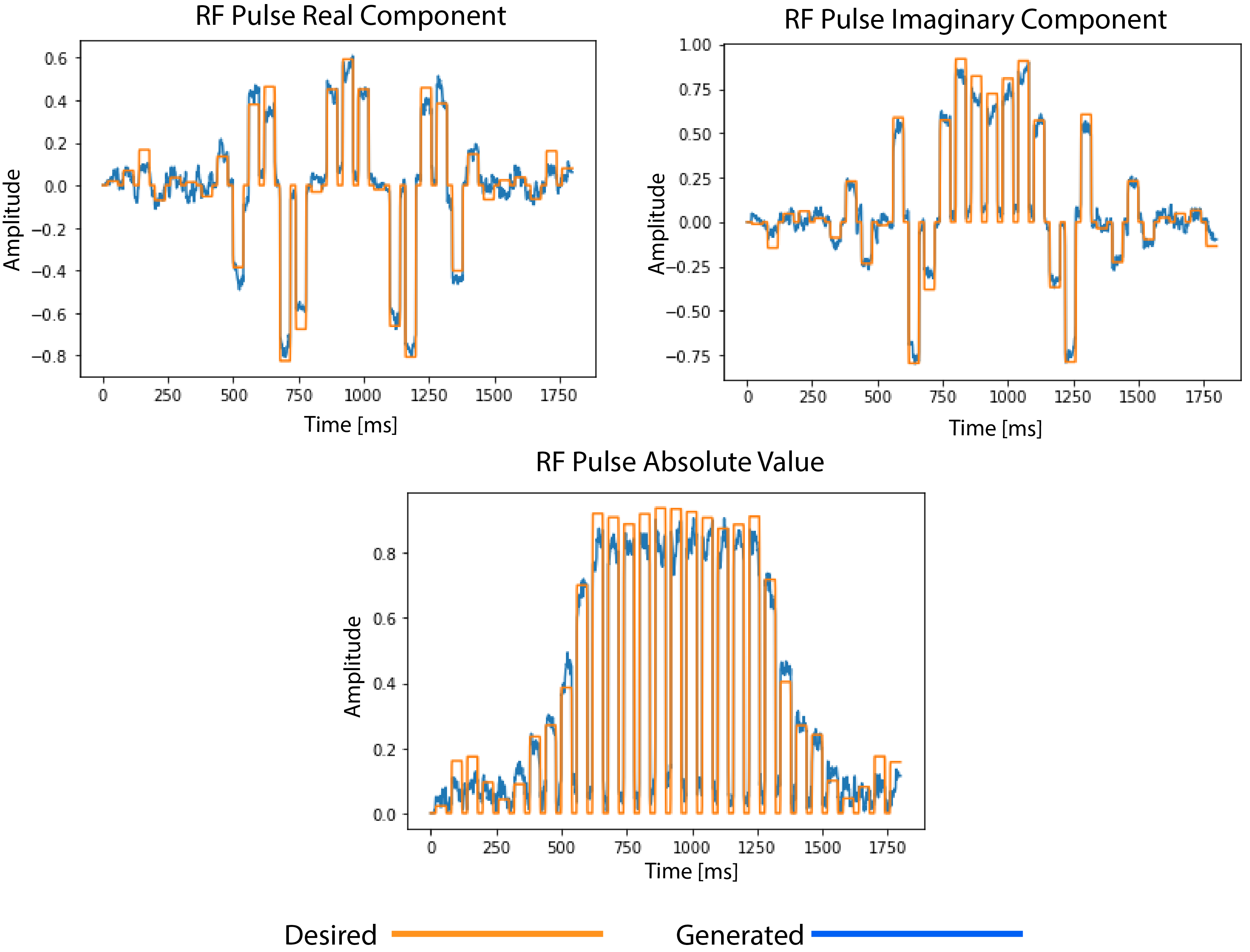
Loss was calculated using mean squared error (MSE). The generated RF real component, imaginary component, absolute value, and gradient overlaid a desired output is shown in Figure 4. We found that although the model was able to generate pulses in response to a desired spatial profile selected to be similar to those used in the training data, it failed when there were significant changes to the input, such a reversal of the ratio between slices. In addition to this, the process to reverse the generated pulses to the spatially simulated pulses returned poor results. Clean spatial magnetization profiles have not yet been obtained. We plan to explore how the fluctuations of the generated pulses, as well as the interpolation of the pulses in order to normalize the training data could affect the spatial simulation.Conclusion
In conclusion, this model serves as a proof of concept for the goal of this project. We will be exploring further investigations such as optimizing the given model, exploring other similar models, and generating a larger and more diverse training dataset.Acknowledgements
No acknowledgement found.References
Feldman RE, Islam HM, Xu J, Balchandani P. A SEmi-Adiabatic matched-phase spin echo (SEAMS) PINS pulse-pair for B1 -insensitive simultaneous multislice imaging. Magn Reson Med. 2016 Feb;75(2):709-17. doi: 10.1002/mrm.25654. Epub 2015 Mar 10. PMID: 25753055; PMCID: PMC4979355.
Norris DG, Koopmans PJ, Boyacioğlu R, Barth M. Power Independent of Number of Slices (PINS) radiofrequency pulses for low-power simultaneous multislice excitation. Magn Reson Med. 2011 Nov;66(5):1234-40. doi: 10.1002/mrm.23152. Epub 2011 Aug 29. PMID: 22009706.
Balchandani P, Pauly J, Spielman D. Designing adiabatic radio frequency pulses using the Shinnar-Le Roux algorithm. Magn Reson Med. 2010;64(3):843-851. doi:10.1002/mrm.22473
Shao J, Ghodrati V, Nguyen KL, Hu P. Fast and accurate calculation of myocardial T1 and T2 values using deep learning Bloch equation simulations (DeepBLESS). Magn Reson Med. 2020;84(5):2831-2845. doi:10.1002/mrm.28321
J. Shao, V. Ghodrati, K.-L. Nguyen, and P. Hu. Fast and accurate calculation of myocardial T1 and T2 values using deep learning Bloch equation simulations (DeepBLESS). Magnetic Resonance in Medicine. 2020;84(5):2831–2845.
Paszke A, Gross S, Massa F, et al. PyTorch: An Imperative Style, High-Performance Deep Learning Library. In: Advances in Neural Information Processing Systems 32. Curran Associates, Inc.; 2019:8024–8035. http://papers.neurips.cc/paper/9015-pytorch-an-imperative-style-high-performance-deep-learning-library.pdf
Figures