2913
Conductivity mapping at 0.55 T with balanced steady state free precession1Department of Radiology, University Hospital Basel, Basel, Switzerland, 2Department of Biomedical Engineering, University of Basel, Basel, Switzerland
Synopsis
Conductivity mapping depends sensitively on the signal-to-noise ratio (SNR) of the transmit phase estimation. It is thus questionable, whether conductivity mapping can be performed at low field. Due to reduced off-resonances, however, a possible solution for the reduced SNR might be offered by balanced steady state free precession (bSSFP). Brain conductivity mapping with bSSFP was investigated at 0.55 T and appears to be feasible but besides SNR also the reduced curvature of the transmit field becomes challenging.
Introduction
Conductivity mapping is based on an estimation of the transmit phase, frequently assessed using the so-called transceive phase assumption1. Generally, the Laplacian calculus in the reconstruction process requires high SNR and therefore electrical properties tomography (EPT) is typically performed at high field strengths. However, lower fields possibly provide many benefits for mapping the conductivity of tissues: on the one hand, the transceive phase assumption is more accurate due to reduced scatter fields and, on the other hand, phase-only conductivity reconstruction becomes a valid simplification due to the lower curvature of the B1+ amplitude1. At high fields, the transceive phase ($$$\varphi^{\pm}$$$) is usually measured with a spin echo. From its refocusing properties, in principle, also balanced steady state free precession (bSSFP) can be used2,3 but accurate transceive phase estimation is limited to its pass-band region. At low field, however, the pass-band region should expand over the whole brain. In this work, we thus explore the feasibility of whole brain conductivity mapping using bSSFP.Methods
For all presented measurements, 3D bSSFP scans were performed on a commercial clinical 0.55 T system (Magnetom FreeMax, Siemens, Erlangen) using a 12-channel head coil for reception. Imaging parameters were: TE/TR = 2.5 ms / 5 ms, flip angle of 40°, bandwidth of 465 Hz/px, matrix of 128×96×88, yielding an isotropic resolution of 2 mm. Individual receive coil signals were combined according to the L1-least-squares method suggested by Lee et al4. In addition, 6-fold long-term averaging was performed to increase the overall SNR, especially for the in vivo measurement. Thus, the total scan could be acquired in a reasonable clinical scan time of just under 5 minutes. A saline phantom (2 g/L Nacl/H2O) with an expected conductivity of 0.34 S/m5 was used for validation purposes. The conductivity was reconstructed using the phase only EPT equation1, $$$\Delta\varphi^{\pm}/(2\mu\omega)$$$, where $$$\mu$$$ is the magnetic permeability and $$$\omega$$$ the Larmor frequency. To adjust for errors at tissue boundaries, the Laplacian was estimated by local parabola fitting6 with a window of 7×7×7 voxels. The conductivity was then filtered with a boundary-preserving median filter with a window of 17×17×17 using the bSSFP magnitude6.Results
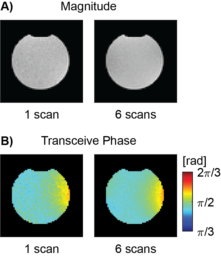
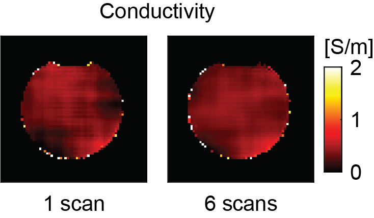
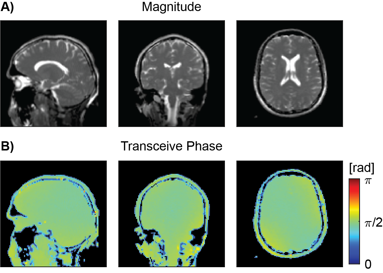
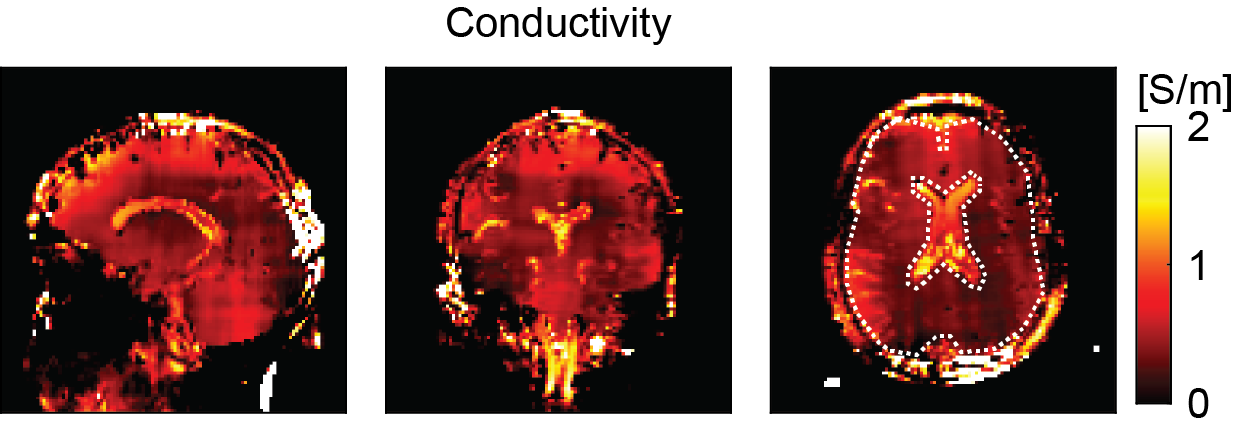
All bSSFP images were essentially free of banding artifacts. Figure 1A and 1B show an example slice of the bSSFP magnitude and phase of the saline phantom measurement from a single scan and averaged over 6 scans. The corresponding reconstructed conductivity images are shown in Figure 2. Restricting conductivity values between 0 and 1, over the whole phantom a mean conductivity of (0.33 ± 0.13) S/m was found for the single scan while the averaged measurement had a value of (0.35 ± 0.13) S/m. Sagittal, coronal and axial bSFFP magnitude and phase images are shown in Figure 3A and 3B, respectively. The corresponding conductivity is shown in Figure 4. A region-of-interest (ROI) is indicated in the axial image for which an average brain tissue conductivity of (0.39 ± 0.19) S/m was found. The distribution of CSF conductivities peaks around the value 1 S/m.Discussion
At 0.55 T, bSSFP provides enough SNR for subsequent conductivity mapping which is mainly due to its increased steady state with decreasing field strength in combination with its property to deliver the highest SNR per unit time among all imaging sequences7. SNR is crucial for proper EPT and even if the SNR at low field can be matched with measurements at high fields with more scan time, the curvature of the transceive phase poses an additional challenge at low field as the Laplacian estimation is more prone to errors. The estimated conductivity of the saline phantom agrees well with the expected value of 0.34 S/m regardless of the averaging. The homogeneity however improved considerably from 1 to 6 scans. Also in the in vivo brain good results are obtained as the obtained value for average brain tissue is close to literature (0.30 S/m)8. CSF conductivity is found to be lower than the expected value of 2.01 S/m8. The difference is mainly attributed to partial volume effects and errors during the magnitude image based reconstruction with a large kernel.Conclusion
In conclusion, despite being challenged by the SNR and low curvature of the transceive phase at low fields, conductivity mapping with bSSFP appears to be feasible at 0.55 T within a clinically acceptable scan time.Acknowledgements
This work was supported by the Swiss National Science Foundation (SNF grant No. 325230_182008).References
1. Lier et al. Electrical Properties Tomography in the Human Brain at 1.5, 3, and 7T: A Comparison Study. Magn. Reson. Med. 2014;71(1):354-363
2. Stehning et al. Real-Time Conductivity Mapping using Balanced SSFP and Phase-Based Reconstruction. Proc. Intl. Soc. Mag. Reson. Med. 19; 2011. Abstract no. 128
3. Stehning et al. Electric Properties Tomography (EPT) of the Liver in a Single Breathhold Using SSFP. Proc. Intl. Soc. Mag. Reson. Med. 20; 2012. Abstract no. 386
4. Lee et al. MR-based conductivity imaging using multiple receiver coils. Magn. Reson. Med. 2016;76(2):530-539
5. Stogryn A. Equations for calculating the dielectric constant of saline water. IEEE Trans. Microwave Theory Tech. 1971;19(8):733-736
6. Katscher et al. Estimation of Breast Tumor Conductivity using Parabolic Phase Fitting. Proc. Intl. Soc. Mag. Reson. Med. 20; 2012. Abstract no. 3482
7. Bieri and Scheffler. Fundamentals of balanced steady state free precession MRI. Magn. Reson. Med. 2013;38(1):2-11
8. Gabriel et al. The dielectric properties of biological tissues: III. Parametric models for the dielectric spectrum of tissues. Phys. Med. Biol. 1996;41(11):2271–2293
Figures