2912
Automatic selection of the optimal kernel size for Helmholtz-based EPT1Istituto Nazionale di Ricerca Metrologica (INRiM), Torino, Italy, 2Department of Radiotherapy, University Medical Center Utrecht, Utrecht, Netherlands, 3Computational Imaging Group for MR Diagnostics & Therapy, Center for Image Sciences, University Medical Center Utrecht, Utrecht, Netherlands
Synopsis
In this work, a procedure for the automatic selection of the optimal kernel size in Helmholtz-based electric properties tomography (MR-EPT) with phase-based approximation is presented and tested on experimental data acquired on a phantom with a 3 T MRI scanner. The procedure is exclusively based on the map of the transceive phase, making no assumptions on the data in addition to those used in the derivation of the Helmholtz-based MR-EPT technique. As a by-product, the approach provides a map indicating the reliability of the reconstructed electric conductivity pixel-by-pixel.
INTRODUCTION
Quantitative imaging of tissue electric properties (EPs) at radiofrequency (RF) could become a useful tool for different clinical applications, because of their alteration in pathological tissues.1,2,3Many techniques have been proposed in the literature to implement the magnetic resonance-based electric properties tomography (MR-EPT).4,5 All of them rely on tunable parameters that help handling the noise in the input data, but whose selection is usually optimized by the user.
Focusing on the phase-based Helmholtz-EPT reconstruction technique,6 an automatic selection of the size of the Savitzky–Golay (SG) filter7 used to compute pixel by pixel the Laplacian of the input data is here described. As a by-product, a map of the trustworthiness of the EPT reconstruction is obtained.
METHODS
The phase-based approximation of Helmholtz-based EPT6 provides an estimate of the electric conductivity distribution $$$\sigma$$$ by elaborating the transceive phase $$$\varphi^\pm$$$ acquired by the MRI scanner according to the relation$$\sigma=\frac{\nabla^2\varphi^\pm}{2\omega\mu_0}\,,$$
where $$$\omega$$$ is the Larmor angular frequency of the system and $$$\mu_0$$$ is the magnetic permeability of vacuum.
The Laplacian of $$$\varphi^\pm$$$ is estimated by applying the SG filter,7 consisting in the local approximation of $$$\varphi^\pm$$$ with the best fitting paraboloid in the least squares sense and the analytical computation of the Laplacian of the resulting surface. Thus, the quality of the recovered conductivity is related to that of the fit.
Working in two dimensions, let us denote the fitting paraboloid by
$$p(x,y)=a_1x^2+a_2y^2+a_3xy+a_4x+a_5y+a_6\,,$$
where $$${\bf a}=[a_k]_{k=1}^6$$$ contains the unknown coefficients determined by minimizing the cost functional
$$F({\bf a})=\sum_{i=1}^m\left\|p(x_i,y_i)-\varphi^\pm_i\right\|^2_2\,.$$
In the latter, $$$m$$$ is the number of points in the SG kernel, whose coordinates are $$$(x_i,y_i)$$$, and $$$\varphi_i^\pm$$$ are the observed transceive phase values.
Being $$${\bf a}^*$$$ the optimal coefficients, the quality of the fit can be measured by the normalized residual sum of squares, that is, by the reduced chi-square statistic
$$\chi^2=\frac{F({\bf a}^*)}{m-6}\,.$$
The normalization with respect to the number of degrees of freedom of the regression problem allow comparing the results obtained with kernels of different sizes.
By estimating the conductivity and the $$$\chi^2$$$ maps with different SG kernels, it is possible to hybridize the results by selecting at each pixel the conductivity value physically admissible (i.e., positive and, possibly, lower than a certain threshold) estimated with the lower $$$\chi^2$$$.
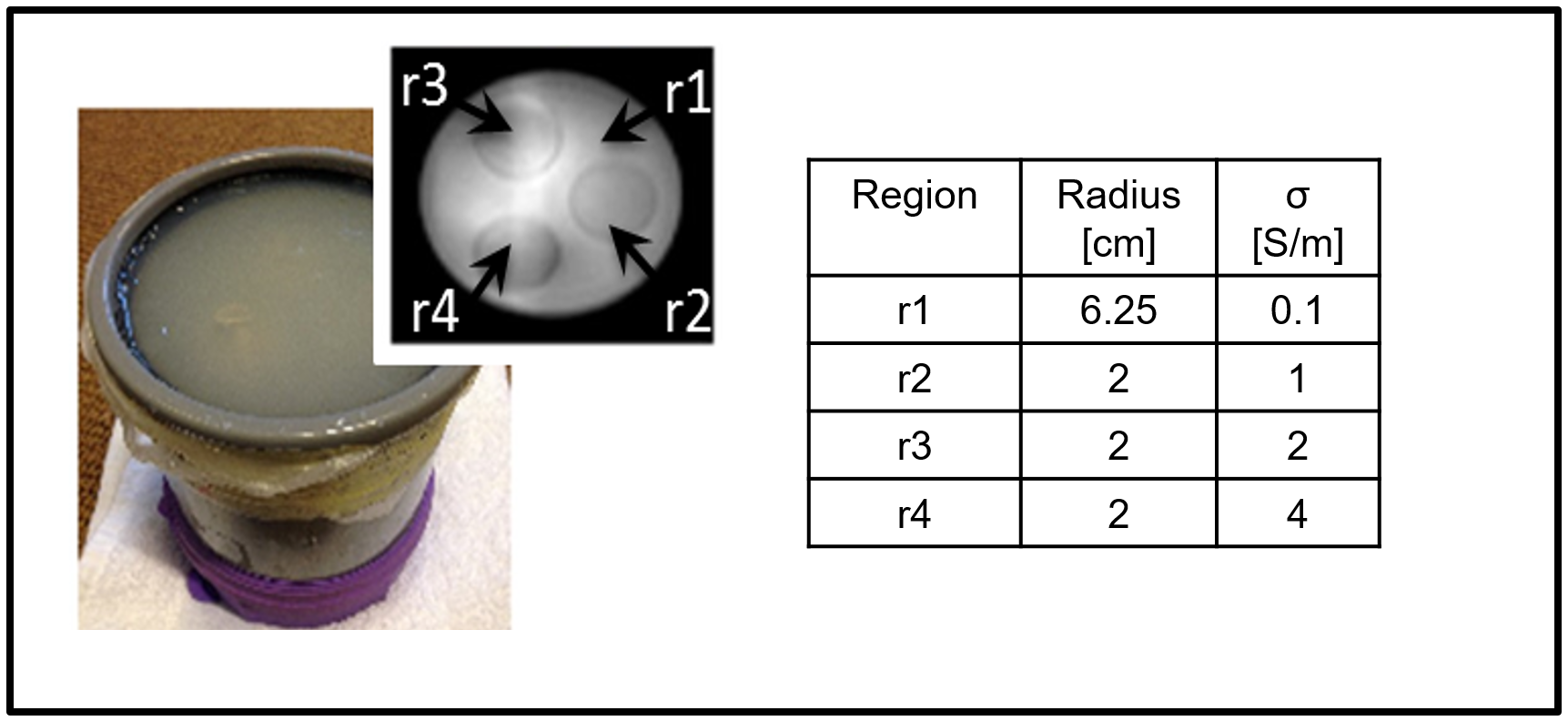
The described procedure is tested on phantom MRI measurements performed using a 3 T scanner (Ingenia, Philips HealthCare, Best, The Netherlands) with the body coil in transmit, and a 15-channel head coil in receive mode. The phantom is cylindrical and agar-based (2 %) with three inner compartments with different amounts of NaCl added to obtain different conductivity values (see Figure 1). Two phase maps acquired using two T1-weighted Spin-Echo sequences with opposite readout gradient polarities were combined to compute $$$\varphi^\pm$$$: TR/TE = 900/5 ms, voxel size = 2x2x2 mm3.
RESULTS
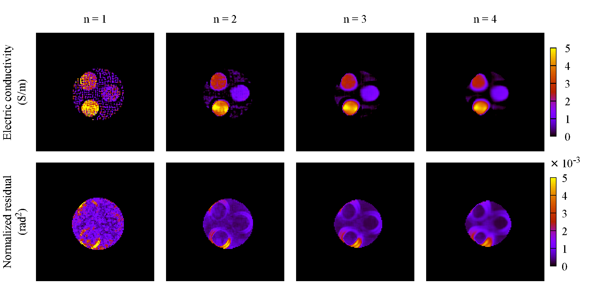
The map of transceive phase $$$\varphi^\pm$$$ acquired on the agar-based phantom is processed by applying the SG filter with a kernel shaped like a square with $$$2n+1$$$ voxels per side. In the following, the value $$$n$$$ is referred to as the kernel size.The distributions recovered by keeping the kernel size constant in the whole image are collected in Figure 2 for $$$n$$$ equal to 1, 2, 3 and 4. The maps of both $$$\sigma$$$ and $$$\chi^2$$$ are reported, the latter being a representation of the trustworthiness of the conductivity estimated in each pixel (the lower $$$\chi^2$$$, the larger the confidence in $$$\sigma$$$).
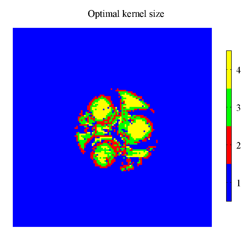
For each pixel, the value of $$$n$$$ which leads to estimate a positive conductivity with the minimum $$$\chi^2$$$ is identified and illustrated in Figure 3. It is worth noting that in the more homogeneous regions (like inside the inclusions) large kernels are selected, whereas small kernels are selected near the boundaries, limiting the inclusion of voxels coming from different regions.
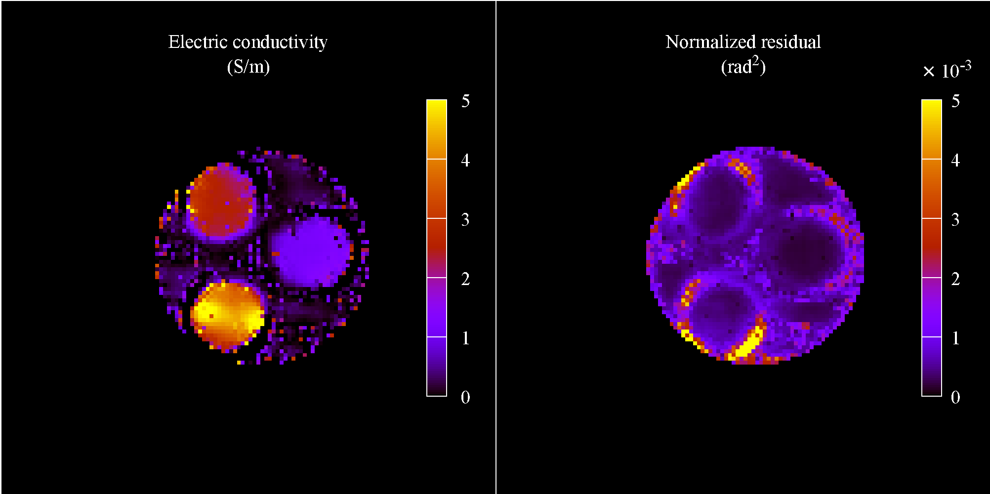
Finally, the maps collected in Figure 2 are hybridized to get the maps of $$$\sigma$$$ and $$$\chi^2$$$ corresponding to the adoption, for each voxel, of the selected optimal kernel size. The resulting reconstructions are shown in Figure 4.
DISCUSSION
The conductivity map obtained with $$$n=1$$$ is significantly affected by noise, but allows to sharply distinguish the different phantom compartments. Instead, the reconstruction provided by $$$n=4$$$ is very smooth, but shows internal boundary errors on wider regions.8 The observed differences are reflected by the $$$\chi^2$$$ map, which identify automatically the internal boundary errors and their extension (see Figure 2).The hybridized reconstruction maintains and combines the positive features of each map reported in Figure 2, keeping low the noise propagation in the estimated conductivity and sharply detecting the internal boundaries (see Figure 4). The $$$\chi^2$$$ map obtained along with the conductivity map provides a useful reference for further processing the data, for example with weighted averaging or median filtering, as well as for a more robust interpretation of the results.
CONCLUSION
A procedure for the automatic selection of the optimal kernel size in Helmholtz-EPT based exclusively on the measured transceive phase map $$$\varphi^\pm$$$ has been proposed.Should analogous quality evaluations be developed also for other MR-EPT reconstruction techniques with an indicator numerically comparable with $$$\chi^2$$$, the proposed procedure could be extended to the hybridization including different techniques, combining advantages of each one of them.
Acknowledgements
The results here presented have been developed in the framework of the 18HLT05 QUIERO project. This project has received funding from the EMPIR programme co-financed by the Participating States and from the European Union’s Horizon 2020 research and innovation programme.
S.M. received funding from NWO, VENI grant n18078.
References
- Tha KK, Katscher U, Yamaguchi S, et al. Noninvasive electrical conductivity measurement by MRI: a test of its validity and the electrical conductivity characteristics of glioma. Eur Radiol. 2018;28(1):348-355. doi:10.1007/s00330-017-4942-5
- Shin J, Kim MJ, Lee J, et al. Initial study on in vivo conductivity mapping of breast cancer using MRI: In Vivo Conductivity Mapping of Breast Cancer. J Magn Reson Imaging. 2015;42(2):371-378. doi:10.1002/jmri.24803
- Kim SY, Shin J, Kim DH, et al. Correlation between conductivity and prognostic factors in invasive breast cancer using magnetic resonance electric properties tomography (MREPT). Eur Radiol. 2016;26(7):2317-2326. doi:10.1007/s00330-015-4067-7
- Leijsen R, Brink W, van den Berg C, Webb A, Remis R. Electrical Properties Tomography: A Methodological Review. Diagnostics. 2021;11(2):176. doi:10.3390/diagnostics11020176
- Arduino A. EPTlib: An Open-Source Extensible Collection of Electric Properties Tomography Techniques. Applied Sciences. 2021;11(7):3237. doi:10.3390/app11073237
- Voigt T, Katscher U, Doessel O. Quantitative conductivity and permittivity imaging of the human brain using electric properties tomography: In Vivo Electric Properties Tomography. Magn Reson Med. 2011;66(2):456-466. doi:10.1002/mrm.22832
- Savitzky A, Golay MJE. Smoothing and Differentiation of Data by Simplified Least Squares Procedures. Anal Chem. 1964;36(8):1627-1639. doi:10.1021/ac60214a047
- Mandija S, Sbrizzi A, Katscher U, Luijten PR, van den Berg CAT. Error analysis of helmholtz-based MR-electrical properties tomography: MR-Electrical Properties Tomography Reconstruction Errors. Magn Reson Med. 2018;80(1):90-100. doi:10.1002/mrm.27004
- Stogryn A. Equations for Calculating the Dielectric Constant of Saline Water (Correspondence). IEEE Trans Microwave Theory Techn. 1971;19(8):733-736. doi:10.1109/TMTT.1971.1127617
Figures