2894
Towards improving high-grade gliomas diagnostic surveillance on T2-weighted images using weak labels from radiology reports1Radiology, Lausanne University Hospital and University of Lausanne, Lausanne, Switzerland, 2Neuroscience Research Center, CHUV, Lausanne, Switzerland, 3Department of Clinical Neurosciences, Lausanne University Hospital and University of Lausanne, Lausanne, Switzerland
Synopsis
Manual annotations are a major bottleneck in supervised machine learning. We present a method that leverages Natural Language Processing (NLP) to generate automatic weak labels from radiology reports. We show how weak labels can be used for the image classification task of high-grade-glioma diagnostic surveillance. We apply a convolutional neural network (CNN) to classify T2w difference maps that either indicate tumor stability or instability. Results suggest that pretraining the CNN with weak labels and fine-tuning it on manually-annotated data leads to better performance (though not statistically significant) when compared to a baseline pipeline where only manually annotated data is used.
1 - Introduction
Diagnostic surveillance aims at monitoring the evolution of a pathology over time to extrapolate clinical knowledge and improve decision-making1. Here, we monitored patients with high-grade gliomas and tried to predict whether there was clinically significant tumor evolution across follow-up sessions. Specifically, we trained a Convolutional Neural Network (CNN) to distinguish difference volumes belonging to the following classes: tumor stability vs. tumor instability (details in 2.1).While Natural Language Processing (NLP) techniques are effective for analyzing radiological reports of oncologic patients2-4, the joint use of radiological reports and images remains under-explored for oncology studies.
In this work, we exploit NLP techniques to obtain weak labels on a large set of unlabeled images. The weak labels are later used to pretrain the CNN for the image classification task. This approach can alleviate the burden of the manual annotation step which is often a major bottleneck in deep learning applications. To the best of our knowledge, this is the first study that assesses the potential of NLP for improving image classification of patients with high-grade gliomas.
2 - Materials and Methods
2.1 DataWe retrieved a retrospective cohort of 181 glioma patients who were scanned between 2004 and 2019 at our university hospital. At every session, a series of MR scans including structural, perfusion and functional imaging were performed. For simplicity, in this work we only focused on the T2w scans. MR acquisition parameters are shown in Figure 1. Also, we extracted the radiology reports associated with each session. These were written (dictated) during routine clinical practice.
Two separate tasks were addressed:
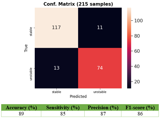
1) Report classification: every report links two MR sessions since the tumor is monitored longitudinally. We applied our report classifier proposed in 4 where an NLP pipeline is trained to distinguish reports that either indicate tumor stability (tumor is unchanged with respect to previous session) or tumor instability (tumor has either worsened or responded to treatment). With respect to the original work 4, we adapted the pipeline to classify the evolution of the lesion on T2-weighted sequences. The NLP pipeline was trained with 215 reports belonging to 123 patients. For each session pair, two independent annotators (with 4 years of experience) tagged the reports with the labels of interest. The 215 reports correspond to the session pairs for which the two annotators agreed.
2) Image classification: each training sample corresponds to a difference map obtained from two time points (two sessions). To obtain these difference volumes, we first registered the previous session to the current session with ANTs5. Then, we skull stripped both volumes (previous warped and current) with FSL-BET6. Third, we applied histogram matching7. Last, we computed the absolute difference between warped and current volume. Figure 2 shows the creation of two difference maps. We divided the image dataset in two groups:
- Human-Annotated Dataset (HAD): this comprises 116 difference maps created from 42 subjects. The gold-standard labels for HAD correspond to those created for the report classification.
- Algorithm-Annotated Dataset (AAD): this comprises 658 difference maps created from 139 distinct subjects. Here, we applied the trained model from 4 to automatically classify the reports, and thus the difference maps. We denote these automatic labels as weak since they are not perfect as they rely on the report classifier performances, but are considerably faster to obtain with respect to the manual ones.
2.2 Experiments
A DenseNet1218 was chosen as CNN for classifying the difference maps. The network was implemented with the Monai framework9. We compared two configurations:
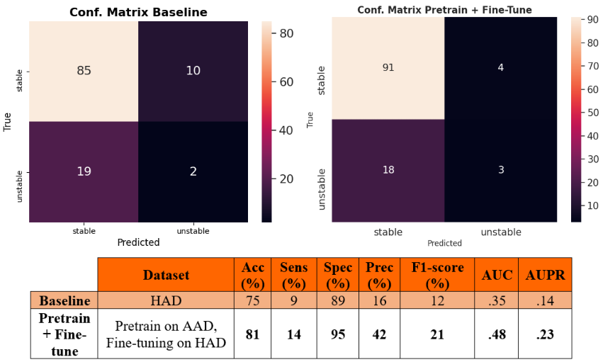
- Baseline: we performed a 5-fold cross-validation on HAD and trained the DenseNet solely on HAD for 75 epochs.
- Pretrain + Fine-tune: we performed once again a 5-fold cross-validation on HAD, but this time we first pretrained the model on AAD (75 epochs), and then fine-tuned it on the HAD train set for 75 epochs.
3 - Results
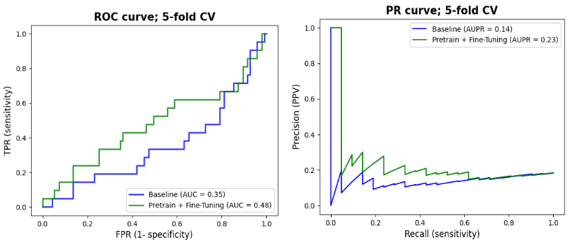
We report in Figure 3 the classification performances of the report classifier that we adapted from 4. Although the model is not perfect, results are well above chance and thus sufficient to automatically create weak labels for the image classification task.Figures 4 and 5 illustrate the results of the difference maps classification (Baseline vs. Pretrain + Fine-tune). The difference in AUC was not statistically significant when performing the permutation test (p=0.3).
4 - Discussion
Results in Figures 4 and 5 show that NLP techniques applied to radiological reports have potential to help for the downstream classification of the difference maps. Although results are preliminary and still too low for clinical utility, the use of NLP to generate weak labels for subsequent machine learning tasks holds noticeable potential since it can alleviate the bottleneck of manual annotation. In future works, we plan to refine the difference maps creation by only focusing on the tumoral region through a pre-segmentation of the scans.Acknowledgements
NoneReferences
- Casey, Arlene, et al. "A systematic review of natural language processing applied to radiology reports." BMC medical informatics and decision making 21.1 (2021): 1-18.
- Chen, Po-Hao, et al. "Integrating natural language processing and machine learning algorithms to categorize oncologic response in radiology reports." Journal of digital imaging 31.2 (2018): 178-184.
- Kehl, Kenneth L., et al. "Assessment of deep natural language processing in ascertaining oncologic outcomes from radiology reports." JAMA oncology 5.10 (2019): 1421-1429.
- Di Noto, Tommaso, et al. "Diagnostic surveillance of high-grade gliomas: towards automated change detection using radiology report classification." medRxiv (2021).
- Avants, Brian B., et al. "A reproducible evaluation of ANTs similarity metric performance in brain image registration." Neuroimage 54.3 (2011): 2033-2044.
- Smith, Stephen M. "Fast robust automated brain extraction." Human brain mapping 17.3 (2002): 143-155.
- Van der Walt, Stefan, et al. "scikit-image: image processing in Python." PeerJ 2 (2014): e453.
- Huang, Gao, et al. "Densely connected convolutional networks." Proceedings of the IEEE conference on computer vision and pattern recognition. 2017.
- MONAI Consortium. (2020). MONAI: Medical Open Network for AI. Zenodo. https://doi.org/10.5281/zenodo.5525502
Figures
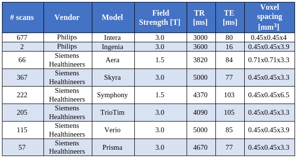
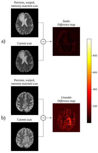
Figure 2.
a) 54-year-old male patient with grade III astrocytoma unchanged (i.e. stable) with respect to the previous session. The difference map is dark in the tumor area.
b) 72-year-old male patient with progressing glioblastoma with respect to the previous session. The enhancing tumor gets highlighted in the difference map. Note that this example is illustrative and most other cases show less pronounced differences between stable and unstable.