Introduction

Continued developments of fast magnetic resonance imaging (MRI) techniques have greatly facilitated speech production studies [1,2]. Sequences of high-quality image volumes are acquired during real-time speech, enabling vocal tract deformation analysis in both visual and quantitative means. Given multiple MRI datasets of a study population, to achieve automated inter-subject comparison, data normalization methods have been proposed including spatial alignment via statistically constructed dynamic image atlases [3,4] and temporal alignment via additional time stamp data processing [5,6]. However, when comparing image data across different speech tasks, manual assessment remains the only reliable method due to the following reasons: 1) four-dimensional (4D) vocal tract shape during different pronunciations varies intensely both in deformation pattern and in temporal length and 2) direct numerical subtraction between image volumes in different tasks is meaningless because unique motion characteristics are hidden in the entire 4D deformation sequence. In this work, we apply an automated two-layer principal component analysis (PCA) to 4D MRI atlases in multiple speech tasks. The first layer extracts the common motion features across different tasks and the second layer extracts unique features of any specific speech utterance. Hidden motion characteristics are automatically separated and revealed by the two layers of principal components (PCs).

Methods

Multi-subject MRI data from a reference speech task and a comparison speech task are acquired. Two sets of 4D dynamic image atlases are constructed using previously proposed method [4] from four healthy subjects’ temporally aligned datasets [6], yielding one image sequence $$$\{I_r(\mathbf{X},t)\},1 \leq t \leq T$$$ for the reference task and another image sequence $$$\{I_c(\mathbf{X},t)\},1 \leq t \leq T$$$ for the comparison task. Note that during atlas construction one specific subject’s anatomy is used as a spatial reference so that $$$\mathbf{X}$$$ in both atlases is the same 3D location. Both sequences are temporally aligned so that $$$t$$$ in both atlases spans the same temporal length $$$T$$$. We use diffeomorphic image registration [7] to extract the deformation fields $$$\{\mathbf{d}_r(\mathbf{X},t)\},2 \leq t \leq T$$$ between every $$$I_r(\mathbf{X},t)$$$ and $$$I_r(\mathbf{X},1)$$$. The same procedure is performed for $$$\{\mathbf{d}_c(\mathbf{X},t)\},2 \leq t \leq T$$$. PCA is used to reveal the maximum differences in a dataset. We perform the first layer of PCA on the deformations $$$\{\mathbf{d}_r(\mathbf{X},t)\}$$$, resulting in $$$\{\mathbf{e}_r^1(\mathbf{X}),...,\mathbf{e}_r^{T-2}(\mathbf{X})\}$$$ showing $$$T-2$$$ principal directions of deformation differences during the reference task. To achieve numerical comparison between the two speech tasks, the second PCA is not performed on the comparison data itself which would result in another intra-task PC decomposition. Instead, the comparison data is modified by subtracting off its “common” motion characteristics to the reference task, i.e., its projections onto the first layer of PC space [8]. Note that the first PCA has centered the reference data by subtracting the mean of all deformations $$$\bar{\mathbf{d}_r}(\mathbf{X})=\sum_t\mathbf{d}_r(\mathbf{X},t)/(T-1)$$$. We need to center the comparison data by $$$\tilde{\mathbf{d}_c}(\mathbf{X},t)=\mathbf{d}_c(\mathbf{X},t)-\bar{\mathbf{d}_r}(\mathbf{X})$$$. The projection $$$p(\tilde{\mathbf{d}_c}(\mathbf{X},t))=(\tilde{\mathbf{d}_c}(\mathbf{X},t) \cdot \mathbf{e}_r^1(\mathbf{X}))\mathbf{e}_r^1(\mathbf{X})+...+(\tilde{\mathbf{d}_c}(\mathbf{X},t) \cdot \mathbf{e}_r^{T-2}(\mathbf{X}))\mathbf{e}_r^{T-2}(\mathbf{X})$$$ is subtracted to modify comparison data by $$$\mathbf{d}^\prime_c(\mathbf{X},t)=\tilde{\mathbf{d}_c}(\mathbf{X},t)-p(\tilde{\mathbf{d}_c}(\mathbf{X},t))$$$. Because the first PC space has a rank of $$$T-2$$$ and the entire two speech tasks have $$$2T-3$$$ degrees of freedom, the rest $$$T-1$$$ principal directions can be any orthogonal vectors. However, all “common” features have been subtracted and stored in the first PC space, all remaining components are therefore unique motion characteristics to the comparison speech task. This is the reason the second PCA is considered an additional layer. Specifically, the covariance matrix of $$$\{\mathbf{d}^\prime_c(\mathbf{X},2),...,\mathbf{d}^\prime_c(\mathbf{X},T)\}$$$ are computed and its eigen decomposition yields $$$T-1$$$ vectors $$$\{\mathbf{e}_c^1(\mathbf{X}),...,\mathbf{e}_c^{T-1}(\mathbf{X})\}$$$ indicating the PC directions for task-specific motion pattern. In total, the two-layer PCA process generates a two-layer PC space $$$\{\mathbf{e}_r^1(\mathbf{X}),...,\mathbf{e}_r^{T-2}(\mathbf{X}),\mathbf{e}_c^1(\mathbf{X}),...,\mathbf{e}_c^{T-1}(\mathbf{X})\}$$$ to represent the common and unique motion characteristics, respectively.

Results and Discussion

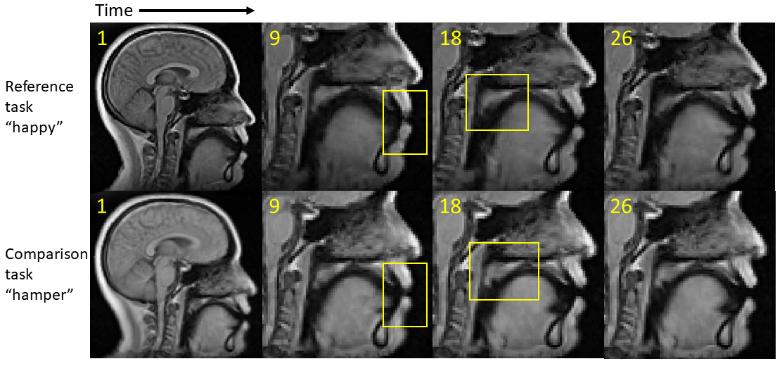
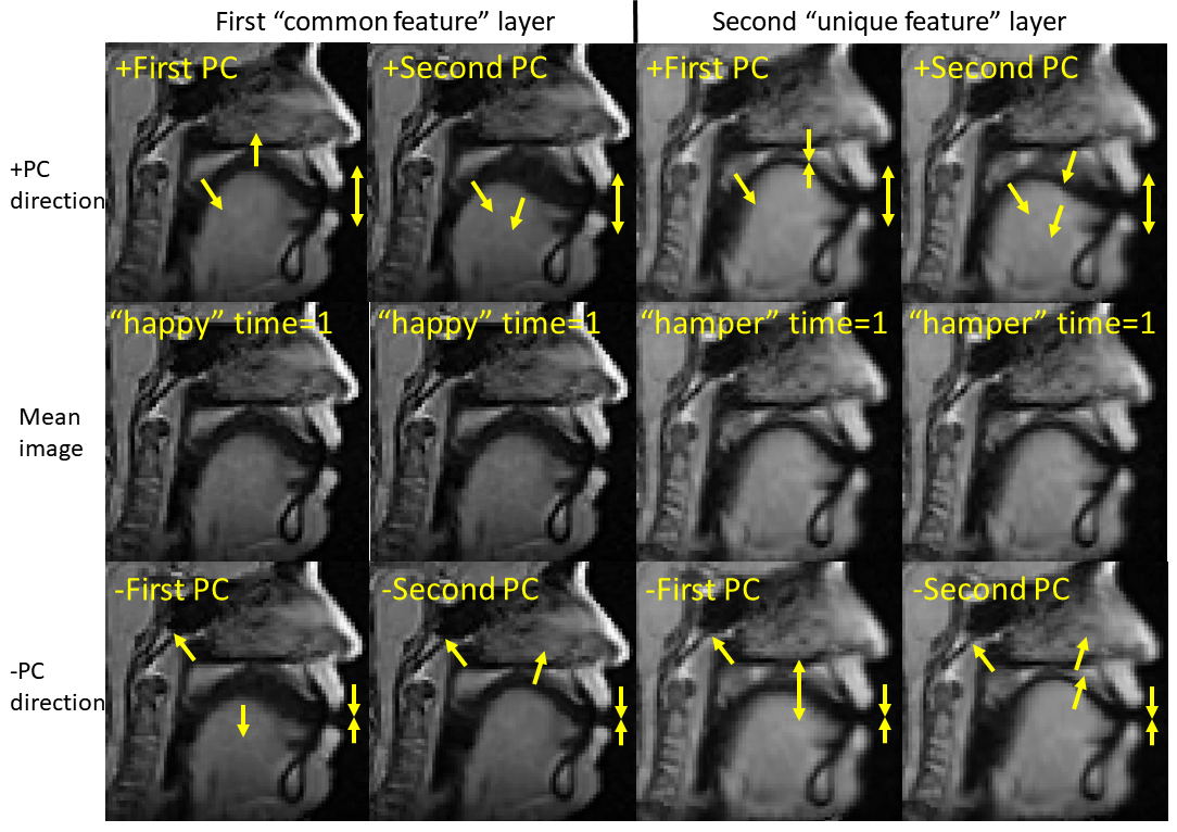
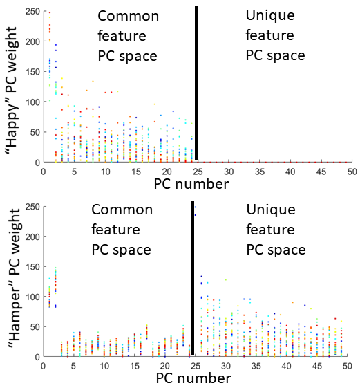
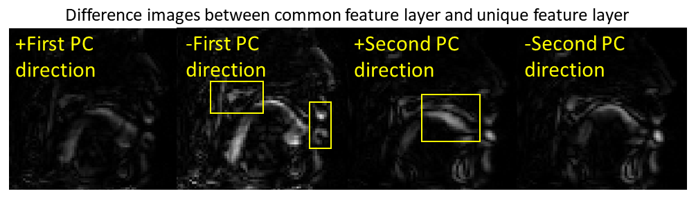
Pronunciation of utterance “happy” was used as reference task with utterance “hamper” as comparison task in our tests. The two sequences of MRI atlases were constructed using the same four subjects within the same space (Fig. 1). Both pronunciations were temporally aligned in $$$T=26$$$ time frames. The two tasks were designed to reflect similar motion patterns with a unique nasal sound /m/ produced in the comparison task. The first layer of 24-dimensional PC space was constructed using “happy” while the second layer of 25-dimensional PC space used “hamper” to extract its unique deformation. The first two PC directions in both spaces containing 66% of all PC weights were used to deform the first image volumes $$$I_r(\mathbf{X},1)$$$ and $$$I_c(\mathbf{X},1)$$$ to reflect their maximum deformation tendency in both the positive and negative principal vector directions (Fig. 2). The projected weights of both tasks on both PC spaces were computed (Fig. 3), showing that the reference task only has weight on the common motion space while the comparison task has weight on both the common space and its unique motion space. Images deformed using unique PCs were subtracted with the common PCs, showing the uniqueness of nasal pronunciation /m/ is mostly in the velopharyngeal port and near the top of the tongue (Fig. 4).

Conclusion

We presented a two-layer PCA on multi-subject speech MRI atlases to automatically extract unique deformation characteristics of the vocal tract in different speech tasks. The analysis quantitatively revealed unique velum and tongue behaviors during nasalization in correspondence to manual assessments.

Acknowledgements

This work was supported by NIH R01DE027989.