Introduction

High resolution diffusion MRI (dMRI) with high b-values is critical for extracting tissue microstructure information. One of the challenges of high-resolution or high b-value dMRI is rectified noise floor. The noise floor can bias the quantification of diffusion metrics from microstructure modeling. Although several advanced dMRI donoising techniques have been proposed ^1,2, they are not good at correcting for this type of noise. Recently we showed that a deep learning based denoising method can reduce noise amplification from Sum-of-Square coil combine mode if using the SENSE1 image as a ground truth ³. Here we show that this method can be used for general denoising, and is very effective in mitigating the noise floor in dMRI.

Methods

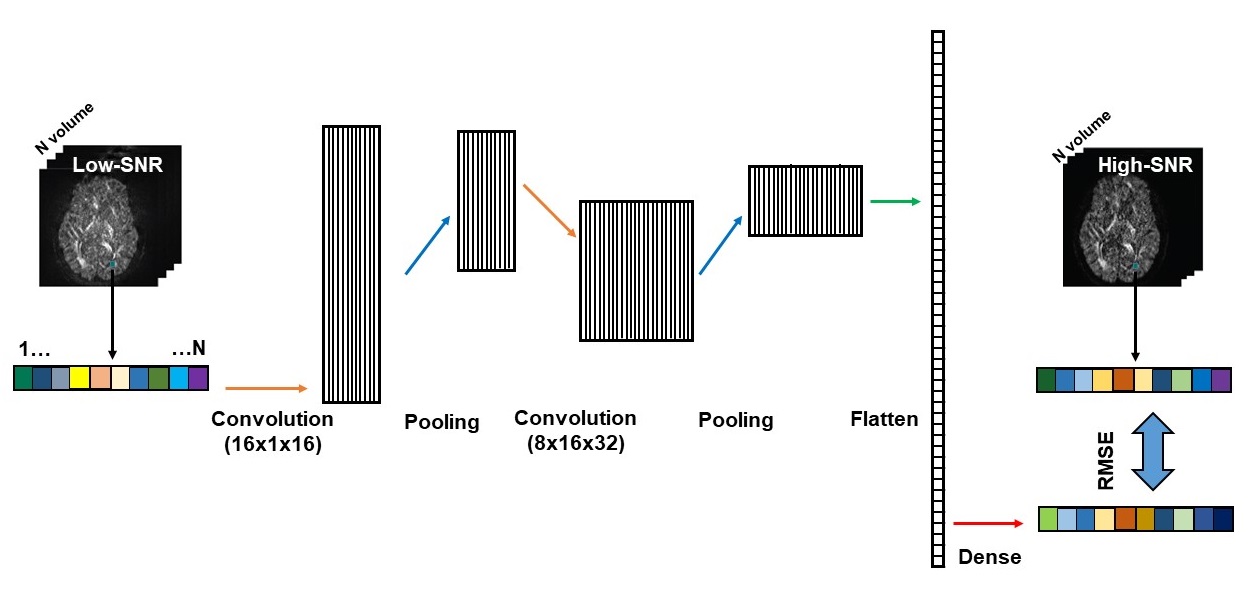
Deep learning network: Inspired by the 1D convolutional neural network for denoising speeches ^4,5, we constructed a simple 1D CNN model that has five layers, including two convolutional layers, each followed by a max-pooling layer, and a dense layer (Fig. 1). The first convolutional layer was fed the low-SNR image and consisted of 16 one-dimensional filtering kernels of size 16. The second convolutional layer consisted of 32 one-dimensional filtering kernels of size 8. The ReLu activation function was used in both convolutional layers. There was 1 max-pooling layer that had a kernel size of 2 with stride 2. In the dense layer, the extracted features of the low-SNR images were mapped to those of the high-SNR images (Fig. 1). The model was implemented in Tensorflow v1.14 and python 3.7.3. The CNN model uses a stochastic gradient descent algorithm for optimization. This model includes several parameters that, in practice, should be optimized for any specific DWI dataset. We used 20000 epochs, learning rate of 0.001, and batch size of 6000 in this study.
Data: We evaluated this method on both simulated data and in vivo data.
Simulation: Four slices of noise-free DWI images were simulated based on the DW-POSSUM framework ⁶, with 4 b0 images, 90 diffusion directions at b-value=1000 s/mm² (b1000) and 90 directions at b-value=2000 s/mm² (b2000). An eight-channel coil model was used to add Gaussian noise to the real and imaginary channel of the data followed by adaptive coil combine, producing two datasets with SNR = 10 and 30, respectively. Two additional datasets with SNR 10 and 30 were generated for testing.
In vivo data: The DWI data of three subjects were acquired on a Prisma scanner using the HCP lifespan protocol: TR/TE = 3470/87 ms, 1.5 mm isotropic resolution, 37 gradient directions with b-value = 1000, 2500 s/mm² plus 6 b0 images, resulting a total of 80 images. We generated two datasets by tweaking the simultaneous multi-slice (SMS) option, one with SMS acceleration factor of 4 (low-SNR) and one without SMS (high-SNR).
Data processing: MPPCA denoising ¹ was applied to simulated dMRI images only, with extent 9×9×3. 1D-CNN were applied to both simulated and in vivo data. For simulated data, the training was between the noisy images and the ground truth. The model obtained from training was applied to the testing datasets. For In vivo data, all images were processed in FSL first for Eddy current/motion correction as well as nonlinear alignment between high-SNR and low-SNR datasets. The training was between the high-SNR and low-SNR images of subject 2 and the model was applied to the other two subjects. Then tensor fitting was performed for all available dMRI datasets to compute fractional anisotropy (FA) and mean diffusivity (MD) using weighted least square option in FSL. The neurite orientation dispersion and density imaging (NODDI) ⁷ analysis was performed using the NODDI Matlab toolbox (http://mig.cs.ucl.ac.uk/index.php). The intra-cellular volume fraction (ICVF) and orientation dispersion index (ODI) were obtained.

Results

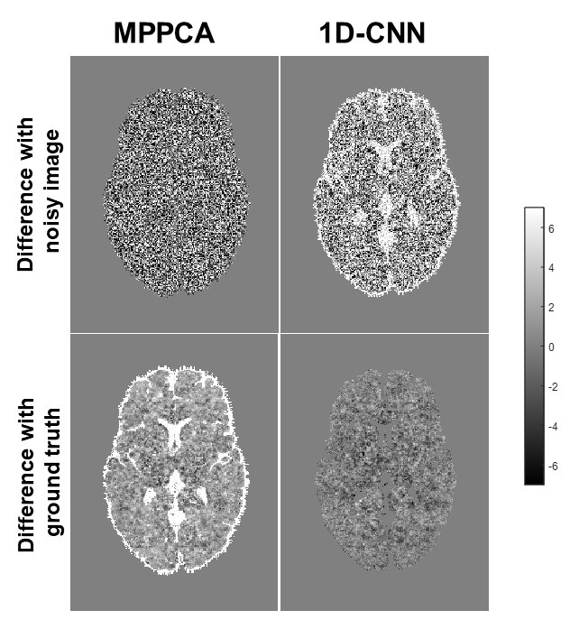
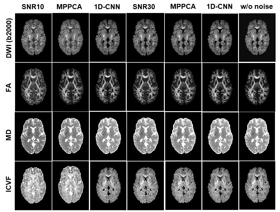
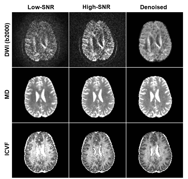
Fig. 2 shows the difference between denoised image and the noisy image as well as the difference between denoised image and the ground truth of a representative slice with b-value 2000 s/mm² from the SNR-10 dataset. MPPCA removed some noise but was unable to restore the signal to the ground truth, as manifested in the CSF region. In contrast, 1D-CNN mapped the noisy image to the ground truth, although the remove noise has some structure. Fig. 3 compares the resultant diffusion metrics of FA, MD, and ICVF for noisy images with SNR 10 and 30, the corresponding denoised images using MPPCA and 1D-CNN, and the ground truth. It shows that the noise floor led to underestimation of FA and MD and overestimation of ICVF substantially as SNR decreases. MPPCA denoising alleviated that effect on FA and MD but not on ICVF. In contrast, 1D-CNN significantly improved the accuracy of MD and ICVF. Similarly, for in vivo data, underestimation of MD and ceiling effect of ICVF were observed for low-SNR data (Fig. 4). 1D-CNN denoising not only revealed more details of the high b-value images but also made MD and ICVF closer to those derived from high-SNR dataset.

Discussion

Both simulation and real data show that the proposed denoising method is robust against noise floor. Since it works on the voxel-wise time course of the dMRI data. even one dMRI dataset will have sufficient samples for training, which is a big advantage in real application.

Acknowledgements

No acknowledgement found.