2815
MRIsim.jl: A framework for end-to-end spin-level MRI simulations with GPU acceleration
Carlos Castillo-Passi1,2,3, Ronal Coronado2,3,4, Sergio Uribe2,3,5, and Pablo Irarrazaval1,2,3,4
1Institute of Biological and Medical Engineering, Pontificia Universidad Católica de Chile, Santiago, Chile, 2Biomedical Imaging Center, Pontificia Universidad Católica de Chile, Santiago, Chile, 3Millennium Nucleus in Cardiovascular Magnetic Resonance, Cardio MR, Santiago, Chile, 4Electrical Engineering, Pontificia Universidad Católica de Chile, Santiago, Chile, 5Radiology Department, School of Medicine, Pontificia Universidad Católica de Chile, Santiago, Chile
1Institute of Biological and Medical Engineering, Pontificia Universidad Católica de Chile, Santiago, Chile, 2Biomedical Imaging Center, Pontificia Universidad Católica de Chile, Santiago, Chile, 3Millennium Nucleus in Cardiovascular Magnetic Resonance, Cardio MR, Santiago, Chile, 4Electrical Engineering, Pontificia Universidad Católica de Chile, Santiago, Chile, 5Radiology Department, School of Medicine, Pontificia Universidad Católica de Chile, Santiago, Chile
Synopsis
In this work, we proposed a GPU-enabled MRI simulation framework written in Julia. The primary purpose of this simulator is to evaluate imaging pipelines from the acquisition to the reconstruction. To showcase this, we simulated two variations of an MRF sequence with radial acquisitions and then reconstructed using two methods. We demonstrated that this framework aids users to quickly write and test state-of-the-art MRI techniques and showed its potential to compare imaging pipelines in quantitative mapping.
Introduction
Numerical simulations are an essential tool to analyze complex systems such as MRI. With MRI simulations, we can isolate and study phenomena by removing unwanted effects. Thus, simulations are ideal for designing pulse sequences, testing reconstruction methods, and creating educational examples.In recent years, researchers have used such tools to generate synthetic data to train Machine Learning (ML) models1 and construct signal dictionaries to infer quantitative measurements from the acquired data2. Regardless, the use of readily available simulators like JEMRIS3, MRISIMUL4, BlochSolver5, MRILab6, coreMRI7, etc is not common practice.
We believe this is due to a lack of open-source simulation frameworks that are fast and written on a high-level programming language, and thus easily extensible. In this work, we developed such a framework using the Julia programming language8.
Methods
Julia programming languageJulia is a language for scientific computing that is fast and has a math-friendly syntax. One of its key advantages is to choose which method of a function to use by multiple dispatch. For example, it is possible to overload an operation, such as addition (+) for a custom object to automatically define array operations.
Objects/Composite types
MRIsim.jl has three main objects:
- Sequence: Gradient waveforms $$$\boldsymbol{G}(t)$$$, RF pulses $$$B_1(t)=B_x(t)+iB_y(t)$$$, and data acquisition timings $$$\text{DAC}(t)$$$.
- Phantom: Representation of the virtual object with properties such as proton density $$$M_0$$$, $$$T_1$$$, $$$T_2$$$, $$$T_2^{*}$$$, off-resonance $$$\Delta\omega$$$, motion $$$\boldsymbol{u}(\boldsymbol{x}_0, t)$$$, postition $$$\boldsymbol{x}_0$$$, etc.
- Hardware: Description of the hardware specifications such as $$$B_0$$$, maximum gradient $$$G_{\max}$$$ and slew rate $$$S_{\max}$$$, non-linearities in the field $$$\Delta B_0(\boldsymbol{x},\boldsymbol{G})$$$, etc.
Simulator
For each spin we simulate the Bloch equation in the rotating frame
$$
\frac{\mathrm{d}\boldsymbol{M}}{\mathrm{d}t}=\gamma\boldsymbol{M}\times\boldsymbol{B}_{\mathrm{eff}}+\frac{\left(M_{0}-M_{z}\right)\hat{\boldsymbol{z}}}{T_{1}}-\frac{M_{x}\hat{\boldsymbol{x}}+M_{y}\hat{\boldsymbol{y}}}{T_{2}},
$$
where $$$\boldsymbol{M}=[M_x,M_y,M_z]$$$ is the magnetization vector and $$$\boldsymbol{B}_{\mathrm{eff}}=[B_x(t),B_y(t),\boldsymbol{G}(t)\cdot(\boldsymbol{x}_0+\boldsymbol{u}(\boldsymbol{x}_0,t))+\gamma^{-1}\Delta\omega]$$$ is the effective magnetic field density.
This equation was solved by using the method of operator splitting12,13. By doing this, we can use the analytical solution of easier problems to update the magnetization vectors.
GPU/CPU parallelization
We parallelized the code using CUDA.jl and the Distributed module. By doing this, we separated the processing of spin-groups to different CPU cores and perform the operations on the GPU.
Graphical User Interface (GUI)
A GUI was also developed based on Electron (Blink.jl), enabling the use of web-based technologies like Plotly.js (Video 1).
Experiments
A radial bSSFP sequence was implemented (Figure 2) to acquire signal fingerprints for each pixel, and a dictionary was generated with the following ranges of $$$T_1$$$ and $$$T_2$$$ values: $$$T_1$$$ (300 to 2.500 ms, every 10 ms) and $$$T_2$$$ (40 to 350 ms, every 4 ms). The simulation was performed using 6.506 spins and 693.535 time-steps ($$$\Delta t=25\,\mu\text{s}$$$ and $$$T=17.3\,\text{s}$$$) in a computer with an 11th Gen Intel i7-1165G7 (8) @ 4 and an NVIDIA GeForce GTX 1650 Ti. The Phantom object was a 2D axial brain constructed using the BrainWeb database14,15. Two sequences were tested, rotating the spokes uniformly ($$$N_{\mathrm{spokes}}=158$$$) and by the golden angle.
Then, the tissue property maps were obtained by performing one of the following reconstruction methods:
- Full-Dict: Filtered back-projection reconstruction for each TR, and then select the closest dictionary entry by using the maximum dot product.
- LRTV: Low-rank dictionary matching with Total variation regularization, with a reduced dictionary of rank 5[16,17,18].
Results
Sequence generationDue to the defined operations between objects, we can easily create the Sequence for the MRF acquisition (Figure 2) by doing the following:
$$
\text{MRF = INV + sum([A[n]*EX + TE[n] + rotz((n-1)*$\Delta\phi$)*RAD + TR[n] for n=1:NTRs]),}
$$with INV the inversion pulse, EX the excitation pulse, TE[n] and TR[n] the corresponding delays, and RAD the radial acquisition. Note that the multiplication of A[n]$$$\in\mathbb{C}$$$ with a Sequence rotates and scales the RF pulses while the multiplication with a matrix $$$\text{rotz((n-1)*$\Delta\phi$)}$$$ rotates the gradient waveforms.
Signal simulation
The whole simulation was only 25 lines of code and took approximately 2 hours. A code-snippet is presented below:
$$
\begin{align*}\mathrm{simParams} & \mathrm{=Dict(:step=>"uniform",:\Delta t=>25e-6,:Nblocks=>20*NTRs)\}}\\\mathrm{recParams} & \mathrm{=Dict(:skip\_{r}ec=>true)}\\\mathrm{signal} & \mathrm{=MRIsim.simulate(phantom,seq,simParams,recParams)}\end{align*}
$$
The acquired signal per TR can be seen in Figure 3.
Reconstruction
The results of the reconstructions are shown in Figure 4. The best overall pipeline was to rotate the spokes by the golden angle and then reconstruct using LRTV, which had MAE's of (WM-T1, GM-T1, WM-T2, GM-T2)=(55,26,15,13) ms.
Conclusions
In this work, we developed an MRI simulation framework enabling rapid prototyping of MRI sequences. This simulator can be used to assess imaging pipelines from the acquisition to the reconstruction. To illustrate this, we tested two reconstruction methods on two MRF sequences to evaluate the quality of the quantitative maps. Our experiments showed that rotating the spokes by the golden angle and using the LRTV reconstruction was the best imaging pipeline. Even though we showed an application in MRF, the simulator can be used in other challenging scenarios and we strongly encourage the involvement of the community to generate new examples and use cases.Acknowledgements
This work was funded by ANID – Millennium Science Initiative Program – NCN17_129.References
- A. S. Lundervold and A. Lundervold, “An overview of deep learning inmedical imaging focusing on MRI,” Zeitschrift für Medizinische Physik,vol. 29, pp. 102–127, May 2019.
- D. Ma, V. Gulani, N. Seiberlich, K. Liu, J. L. Sunshine, J. L. Duerk, andM. A. Griswold, “Magnetic resonance fingerprinting,” Nature, vol. 495, pp. 187–192, Mar. 2013.
- T. Stocker, K. Vahedipour, D. Pflugfelder, and N. J. Shah, “High-performance computing MRI simulations,” Magnetic Resonance in Medicine, vol. 64, no. 1, pp. 186–193, 2010.
- C. G. Xanthis, I. E. Venetis, A. V. Chalkias, and A. H. Aletras,“MRISIMUL: A GPU-Based Parallel Approach to MRI Simulations,” IEEE Transactions on Medical Imaging, vol. 33, pp. 607–617, Mar.2014.
- R. Kose and K. Kose, “BlochSolver: A GPU-optimized fast 3D MRIsimulator for experimentally compatible pulse sequences,” Journal of Magnetic Resonance, vol. 281, pp. 51–65, Aug. 2017.
- F. Liu, J. V. Velikina, W. F. Block, R. Kijowski, and A. A. Samsonov, “Fast Realistic MRI Simulations Based on Generalized Multi-Pool Ex-change Tissue Model,” IEEE Transactions on Medical Imaging, vol. 36, pp. 527–537, Feb. 2017.
- C. G. Xanthis and A. H. Aletras, “coreMRI: A high-performance, publicly available MR simulation platform on the cloud,” PLOS ONE, vol. 14, p. e0216594, May 2019.
- J. Bezanson, A. Edelman, S. Karpinski, and V. B. Shah, “Julia: A fresh approach to numerical computing,” SIAM review, vol. 59, no. 1, pp. 65–98, 2017.
- K. J. Layton, S. Kroboth, F. Jia, S. Littin, H. Yu, J. Leupold, J.-F.Nielsen, T. Stöcker, and M. Zaitsev, “Pulseq: A rapid and hardware-independent pulse sequence prototyping framework,” Magnetic Resonance in Medicine, vol. 77, no. 4, pp. 1544–1552, 2017.
- K. S. Ravi, S. Potdar, P. Poojar, A. K. Reddy, S. Kroboth, J.-F. Nielsen, M. Zaitsev, R. Venkatesan, and S. Geethanath, “Pulseq-Graphical Programming Interface: Open source visual environment for prototyping use sequences and integrated magnetic resonance imaging algorithm development,” Magnetic Resonance Imaging, vol. 52, pp. 9–15, Oct.2018.
- S. J. Inati, J. D. Naegele, N. R. Zwart, V. Roopchansingh, M. J. Lizak,D. C. Hansen, C.-Y. Liu, D. Atkinson, P. Kellman, S. Kozerke, H. Xue, A. E. Campbell-Washburn, T. S. Sørensen, and M. S. Hansen, “ISMRMRaw data format: A proposed standard for MRI raw datasets,” MagneticResonance in Medicine, vol. 77, pp. 411–421, Jan. 2017.
- A. Hazra, G. Lube, and H.-G. Raumer, “Numerical simulation of Blochequations for dynamic magnetic resonance imaging,” Applied NumericalMathematics, vol. 123, pp. 241–255, Jan. 2018.
- C. Graf, A. Rund, C. S. Aigner, and R. Stollberger, “Accuracy and performance analysis for Bloch and Bloch-McConnell simulation methods,” Journal of Magnetic Resonance, vol. 329, p. 107011, Aug. 2021.
- B. Aubert-Broche, A. C. Evans, and L. Collins, “A new improved version of the realistic digital brain phantom,” NeuroImage, vol. 32, pp. 138–145, Aug. 2006.
- B. Aubert-Broche, M. Griffin, G. B. Pike, A. C. Evans, and D. L. Collins,“Twenty new digital brain phantoms for creation of validation image databases,” IEEE transactions on medical imaging, vol. 25, pp. 1410–1416, Nov. 2006.
- M. Golbabaee, G. Buonincontri, C. Pirkl, M. Menzel, B. Menze,M. Davies, and P. Gomez, “Compressive MRI quantification using con-vex spatiotemporal priors and deep auto-encoders,” arXiv:2001.08746[physics], Apr. 2020.
- J. Assländer, M. A. Cloos, F. Knoll, D. K. Sodickson, J. Hennig, andR. Lattanzi, “Low-Rank Alternating Direction Method of Multipliers Re-construction for MR Fingerprinting,” Magnetic resonance in medicine, vol. 79, pp. 83–96, Jan. 2018.
- J. Fessler and B. Sutton, “Nonuniform fast Fourier transforms using min-max interpolation,” IEEE Transactions on Signal Processing, vol. 51, pp. 560–574, Feb. 2003.
Figures
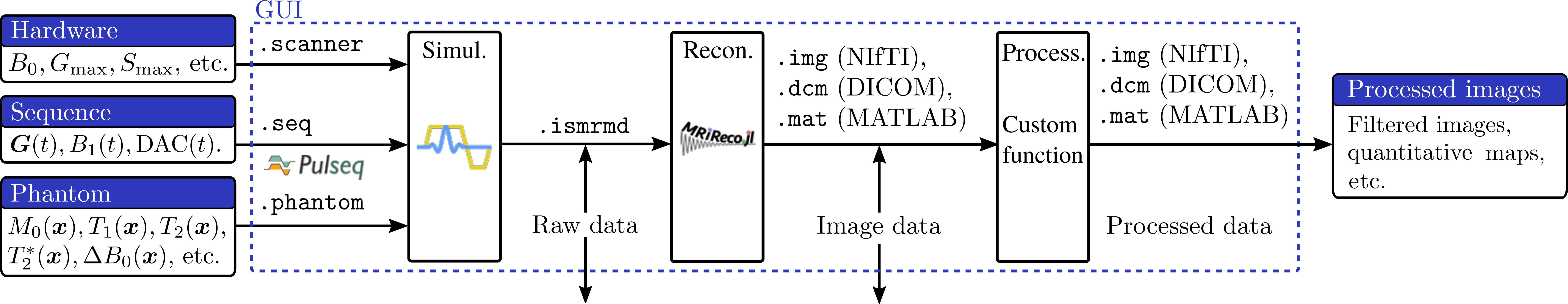
Figure 1. The simulation pipeline is divided into three steps: (1) simulation, (2) reconstruction, and (3) post-processing. Each arrow represents a file, and the pipeline can be initiated from any stage of the data workflow.
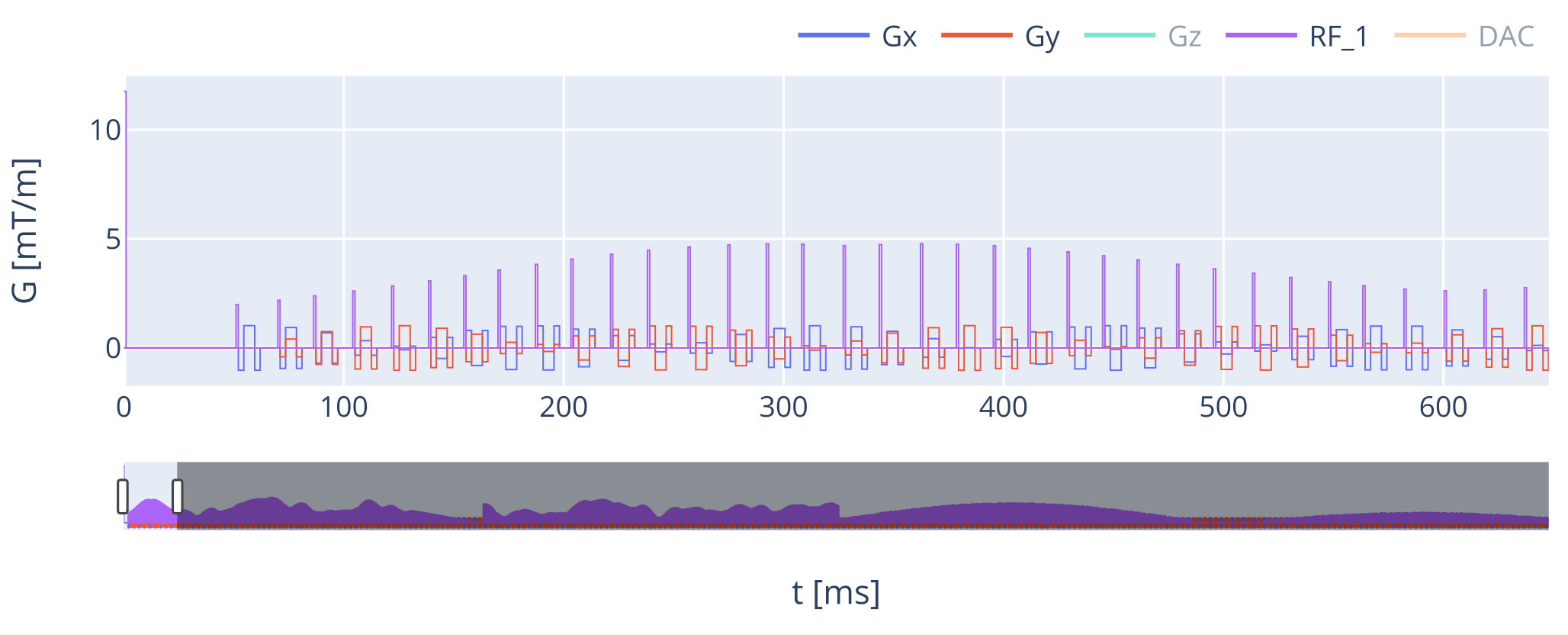
Figure 2. MRF sequence based on a radial bSSFP. The acquisitions were rotated by either using the tiny-golden angle Δθ = 23.6281 deg or Δθ = 1.1392 deg. Each TR had different flip-angles (α), pulse phase (ϕ), and repetition time (TR). The echo time (TE) was constant and set to 5 ms, and the acquisition time (Ta) was also 5 ms. The DAC for each TR had 100 samples.
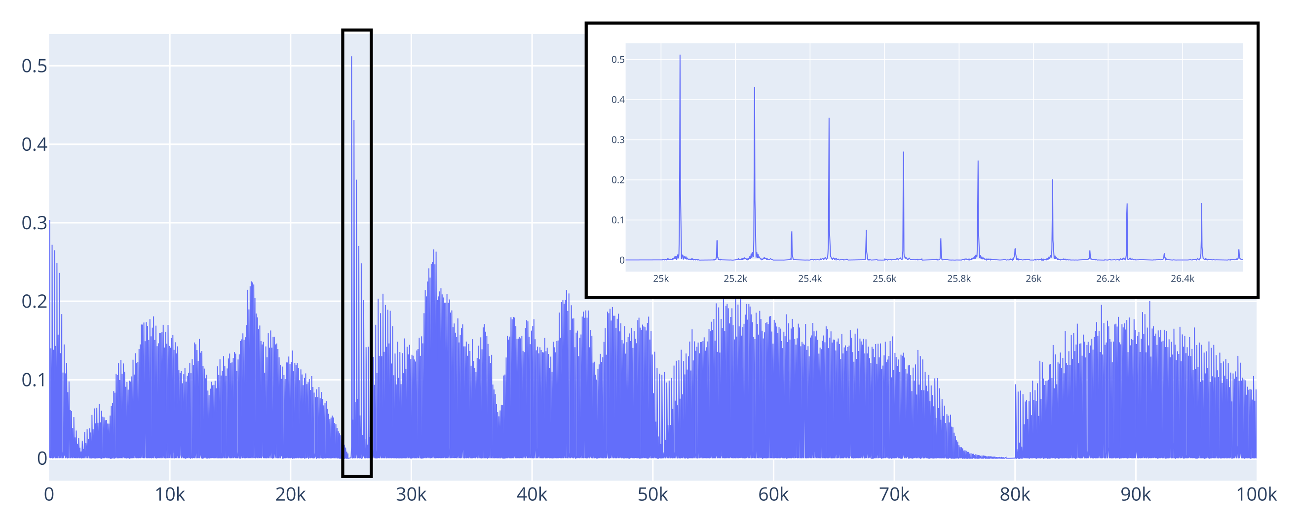
Figure 3. (Left.) The simulated MRF signal and (Right.) a zoom showing the echoes on each TR.
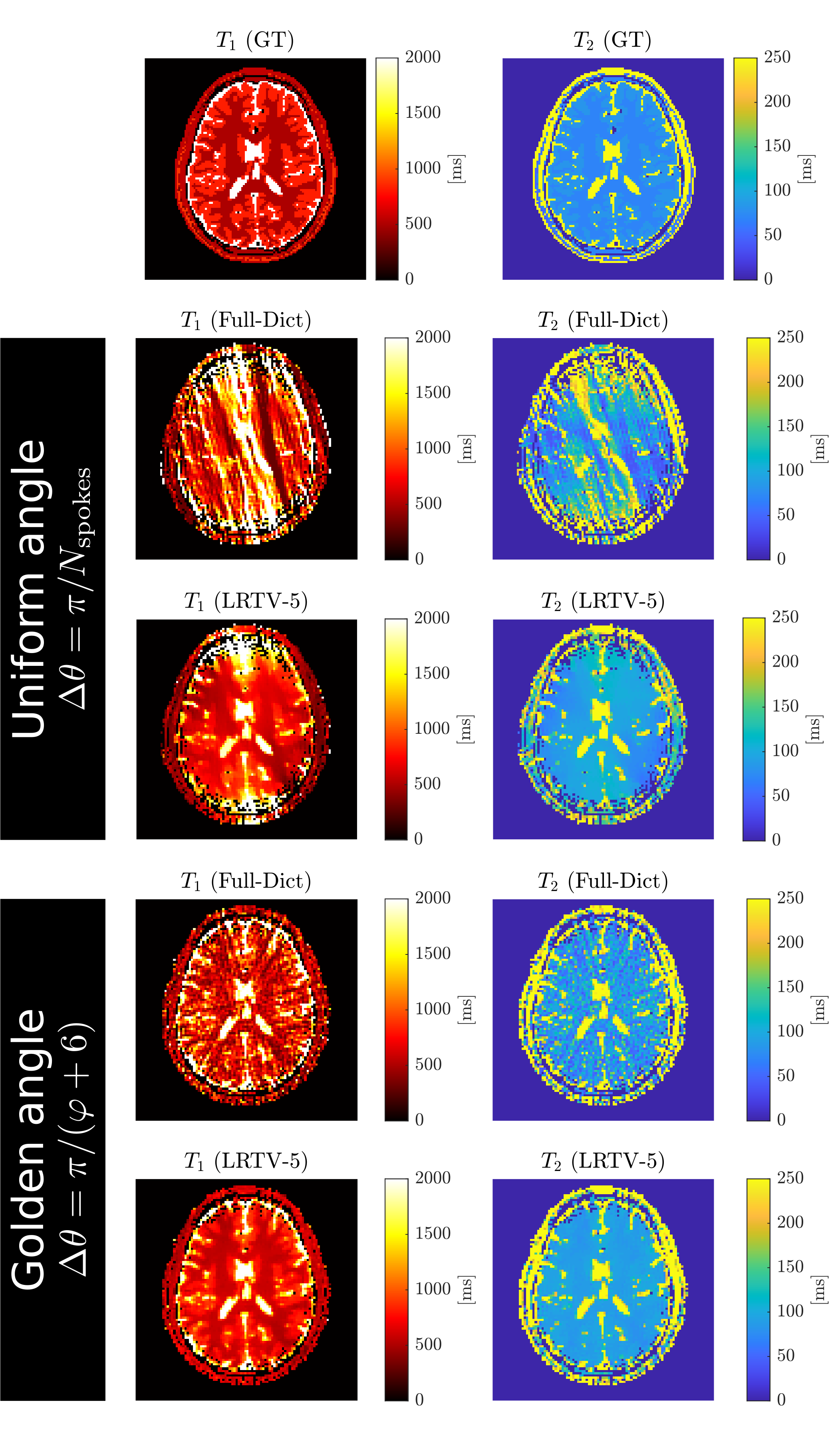
Figure 4. Comparison of the acquisition and reconstruction methods. (GT) Ground-truth, (Full-Dict) reconstruction using the full dictionary, and (LRTV-5) Low-rank with Total Variation reconstruction with rank of 5 for the dictionary.
Video 1 (Click me!). SpinLab GUI demonstration. We show how each tab of the GUI works, by using the default phantom (an axial 2d brain) and sequence (an EPI with TE of 25 ms).
DOI: https://doi.org/10.58530/2022/2815