2810
Towards gradient perturbation correction in diffusion weighted imaging based on the gradient system transfer function1Department of Diagnostic and Interventional Radiology, University of Würzburg, Würzburg, Germany
Synopsis
Eddy current induced field perturbations can cause artifacts in diffusion weighted imaging (DWI). Such perturbations may be calculated and corrected for by the gradient system transfer function (GSTF), provided the gradient system behaves linear and time-invariant. We discovered that the linearity assumption can be violated by gradients with high zeroth order moments. We therefore propose a modified measurement scheme for the GSTF including higher gradient moments to better approximate their behavior. Our approach substantially reduces errors in the predicted gradient time courses. We may thus enable the application of GSTF-based correction methods to DWI in the future.
Introduction
Diffusion weighted imaging (DWI) can suffer from field perturbations caused by eddy currents induced by the MR scanner’s gradient coils, resulting in ghosting artifacts and geometric infidelity. It was previously shown that concurrent field monitoring can mitigate these effects.1 However, this technique requires special hardware. The gradient system transfer function (GSTF) constitutes another convenient tool for mitigating image artifacts arising from distorted gradient waveforms2,3, and can be determined using standard scanner hardware4. Under the assumption that the gradient system acts linear and time-invariant (LTI), the GSTF allows the prediction of the true gradient fields of arbitrary waveforms4. However, nonlinear behavior of the gradient amplifiers5 or temperature effects6,7 may violate this assumption. In this work, we demonstrate the violation of the linearity assumption for gradients with high zeroth order moments, as often employed in DWI. Furthermore, we present a modified approach to measure the GSTF, better approximating the actually produced gradient over a wider range of gradient moments.Methods
We measured all gradient time courses following the thin-slice approach proposed by Duyn et al.8. The measurements were conducted on a 3T Siemens MAGNETOM Prismafit scanner (Siemens Healthcare, Erlangen, Germany) using a 16-channel head coil and a spherical phantom. To determine the present post-pulse gradient field oscillations immediately after switching off (large) trapezoidal gradients with the thin-slice approach, we employed a spin-echo measurement scheme, as depicted in figure 1. We investigated three different trapezoids, one resembling a diffusion-weighting gradient for a high b-value (gradient moment M=627mT/m∙ms), one resembling a single-line-segment of an EPI readout gradient (M=15mT/m∙ms) and one resembling a phase-encoding gradient (M=5mT/m∙ms). The GSTF calculation was based on three measurements, schematically depicted in figure 2. In the first, ten short triangular gradient pulses (M=0.5mT/m∙ms – 3.8mT/m∙ms) were played out while acquiring the FID signal, after a slice-selective excitation, as similarly published before2,3. In the second measurement, ten different, mostly larger, triangles (M=1.2mT/m∙ms – 113mT/m∙ms) were applied, followed by a slice-selective excitation and acquisition of the FID signal9. In the third measurement, the same triangles as in the second measurement were captured with a spin-echo measurement scheme, to record the ramp down of the gradients. Table 1 summarizes the exact measurement parameters. The measurements were combined in a linear system of equations to calculate the GSTF by a matrix inversion7 and Fourier transform. We applied Tikhonov regularization to reduce high frequency noise. Time intervals with dephased signal in measurement three were omitted from the calculation. One GSTF was calculated using only the data from the first measurement (“GSTF 1”). A second GSTF encompassed all three datasets (“GSTF 2”).Results
Figure 3a) and b) display the magnitude and phase of GSTF 1 and 2. The insets provide zoomed views of the low frequency range, where the two curves show variations not related to noise. These appear even more clearly in the difference of both curves in figure 3c) and d). Figure 4 displays the measured progressions of the trapezoidal gradients and the ones predicted with the two different GSTFs. The zoomed inset in figure 4a) shows a distinct discrepancy between the measured large gradient and the prediction based on GSTF 1. The respective RMSE is 9.9∙10-3mT/m. (The gray shaded areas were omitted from the RMSE calculation because the measured signal was dephased there, not allowing to determine the applied gradient.) The predicted gradient based on GSTF 2 in figure 4b) agrees much better with the measured curve, also reflected in the lower RMSE of 4.2∙10-3mT/m. For the smaller trapezoids (figure 4c) – f)), GSTF 1 and 2 yield similar predictions that concur well with the measurements. The respective RMSEs (1.465∙10-2mT/m in figure 4c), 1.463∙10-2mT/m in figure 4d), 2.143∙10-2mT/m in figure 4e), and 2.142∙10-2mT/m in figure 4f)) only differ negligibly.Discussion
The discrepancies between the measured and predicted gradient courses in figure 4a) prove that the gradient system deviates from the LTI assumption when executing long gradients with high amplitudes. Probing the gradient system’s impulse response behavior over a larger range of different gradient moments helps reducing errors in GSTF-based gradient calculations for high moments, as demonstrated by the results in figure 4b). Conventional phantom-based GSTF measurements3 could not include higher moments as they dephase the signal too much. Yet, our approach does not impair GSTF-based gradient predictions of smaller moments, as shown in figure 4c) – f). These important insights pave the way towards applying GSTF-based correction methods in DWI. Although we only show results for the z-gradient, we made similar observations for the same measurements performed on the x- and y-axis. However, these findings may not hold true if a gradient system violates the LTI assumption to a greater extent than ours. In this case, concurrent field monitoring10 or a current-to-field transfer function5 may be viable alternatives to obtain the actual gradient.Conclusion
Our work illustrates the importance to validate the LTI assumption when applying GSTF-based gradient corrections, especially in DWI. We also offer an approach to overcome small deviations from the LTI behavior in the GSTF determination, which is easy to implement, only requiring a phantom and standard scanner hardware. Our findings may thus help to facilitate the correction of spatiotemporal field perturbations in DWI.Acknowledgements
No acknowledgement found.References
1. Wilm BJ, Nagy Z, Barmet C, et al. Diffusion MRI with Concurrent Magnetic Field Monitoring. Magn Reson Med. 2015;74:925-933.
2. Vannesjo SJ, Haeberlin M, Kasper L, et al. Gradient System Characterization by Impulse Response Measurements with a Dynamic Field Camera. Magn Reson Med. 2013;69:583-593.
3. Campbell-Washburn AE, Xue H, Lederman RJ, et al. Real-Time Distortion Correction of Spiral and Echo Planar Images Using the Gradient Impulse Response Function. Magn Reson Med. 2016;75:2278-2285.
4. Addy NO, Wu HH, Nishimura DG. Simple Method for MR Gradient System Characterization and k-Space Trajectory Estimation. Magn Reson Med. 2012;68:120-129.
5. Rahmer J, Schmale I, Mazurkewitz P, et al. Non-Cartesian k-space trajectory calculation based on concurrent reading of the gradient amplifiers’ output currents. Magn Reson Med. 2021;85:3060-3070.
6. Stich M, Pfaff C, Wech T, et al. The temperature dependence of gradient system response characteristics. Magn Reson Med. 2020;83:1519-1527.
7. Wilm BJ, Dietrich BE, ReberJ, et al. Gradient Response Harvesting for Continuous System Characterization During MR Sequences. IEEE Trans Med Imag. 2020;39(3):806-815.
8. Duyn JH, Yang Y, Frank JA, et al. Simple Correction Method for k-Space Trajectory Deviations in MRI. J Magn Reson. 1998;132:150-153.
9. Scholten H, Stich M, Köstler H. Phantom-based high-resolution measurement of the gradient system transfer function. In Proceedings of the 2021 ISMRM Annual Meeting, 2021. Abstract 3087.
10. Barmet C, De Zanche N, Pruessmann KP. Spatiotemporal Magnetic Field Monitoring for MR. Magn Reson Med. 2008;60:187-197.
11. White MJ, Wilkinson T, Gomez D. mr-sequence-diagrams. https://github.com/dangom/mr-sequence-diagrams. Accessed June 25, 2020.
Figures
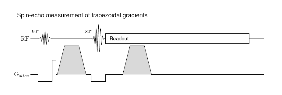
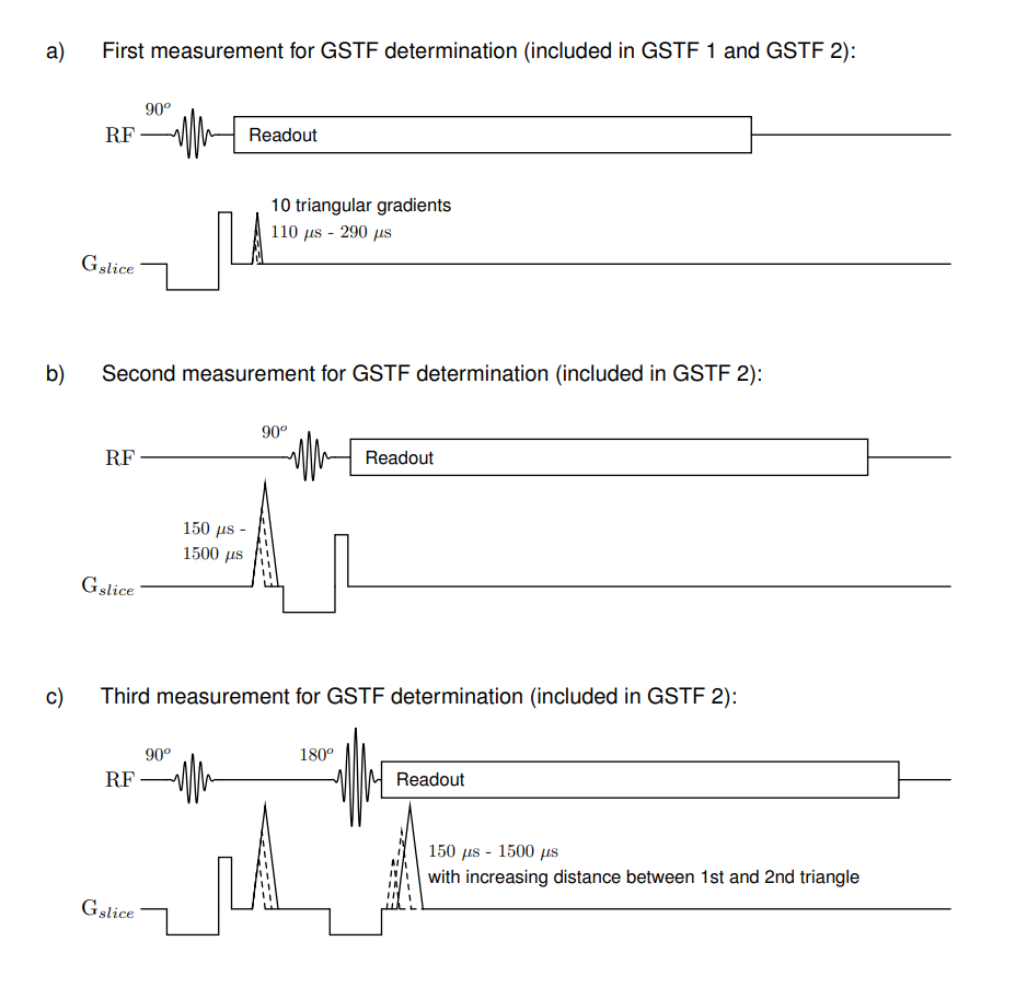
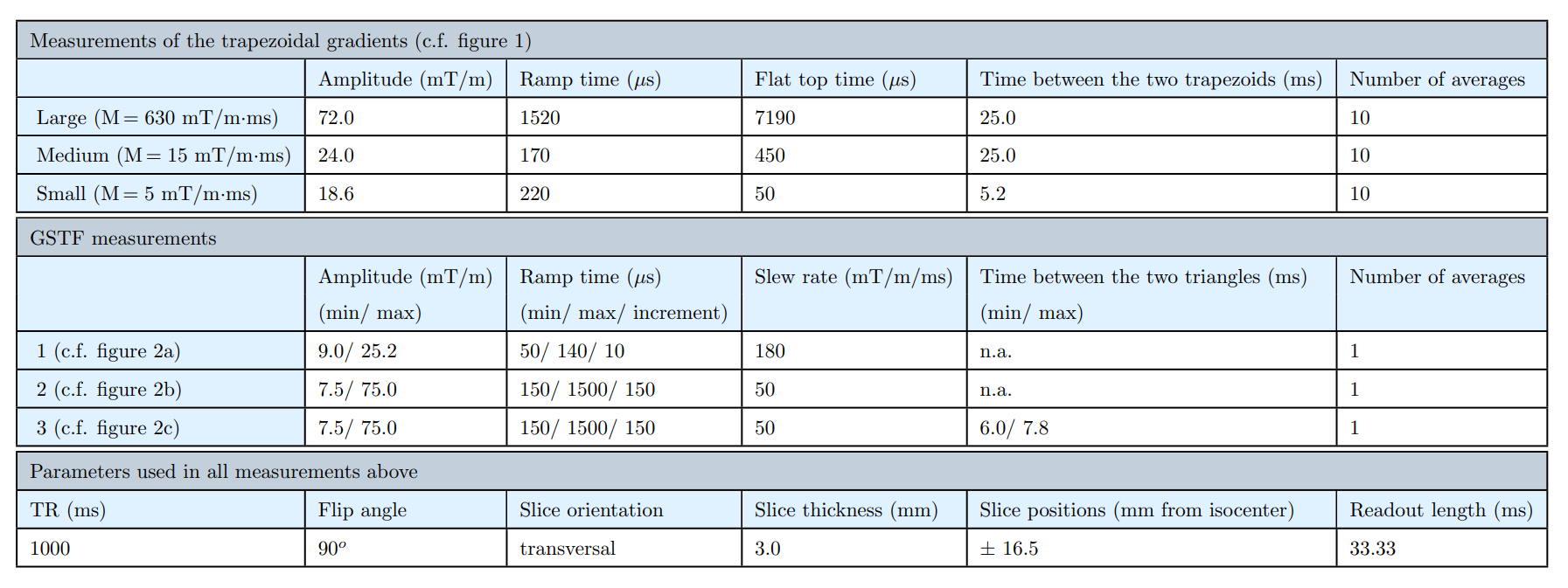
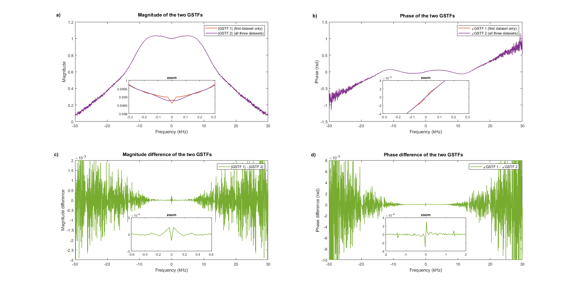
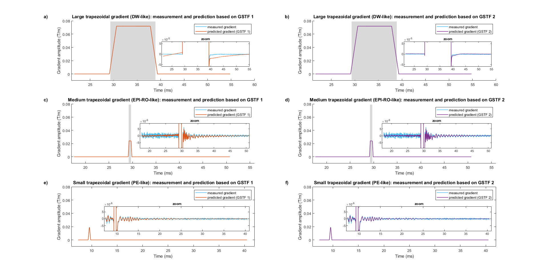
Figure 4: Measured and predicted gradient time courses of trapezoidal gradients. The insets are zoomed on the y-axis to show the differences between the curves. The gray shaded areas mark where the measured signal was dephased, so the gradients’ progressions could not be captured completely. These parts are not plotted here and were omitted from the RMSE calculations.